Next: discussion and conclusion
Up: Tang: Regularized inversion
Previous: diagonal approximation of Hessian
I test my methodology on two synthetic 2-D data sets. One shown in Figure 2(a) is
a two-layer model with one reflector being horizontal and the other dipping at
 . The velocity increases with
depth: v(z) = 2000 + 0.3z, which is shown in Figure 1. To make the
synthetic data set more realistic, some random noise has also been added.
Then I replace approximately
. The velocity increases with
depth: v(z) = 2000 + 0.3z, which is shown in Figure 1. To make the
synthetic data set more realistic, some random noise has also been added.
Then I replace approximately  of the traces in the offset dimension
with zeros. The incomplete and sparse data set is shown in Figure 2(b). Then I perform
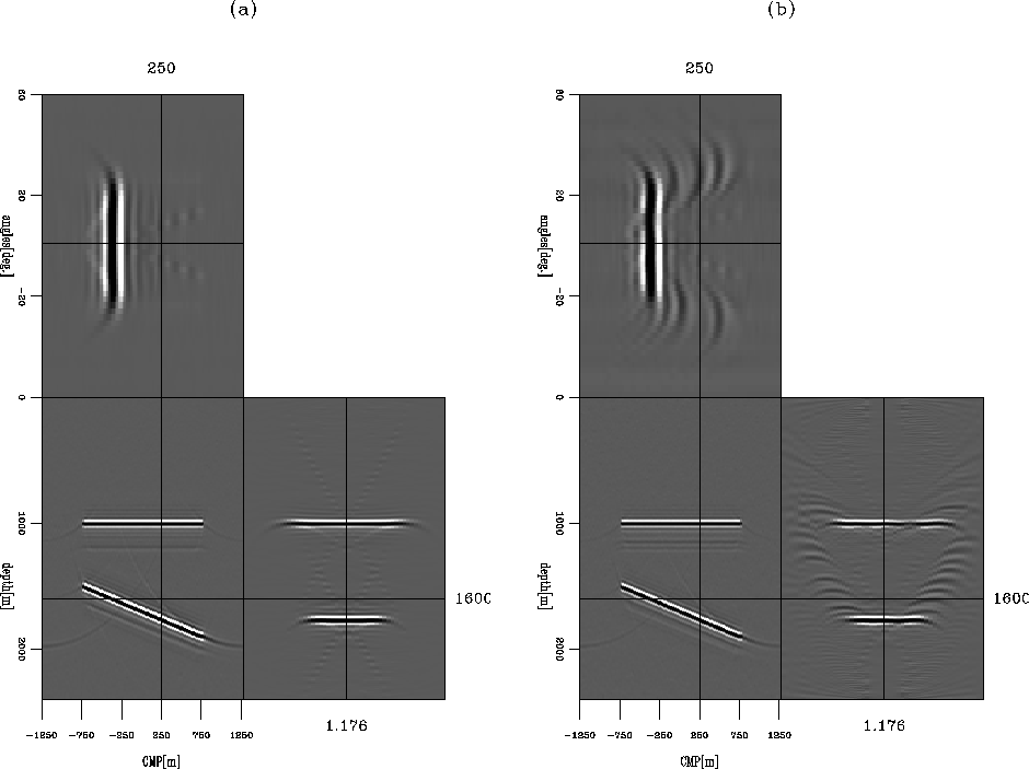
DSR migration on both data sets to generate the SODCIGs; the corresponding migrated image cubes are shown in
Figure 3. Comparing Figure 3(a) with
Figure 3(b), we can see that even with the complete data set (Figure 2(a)),
the SODCIGs suffer from the amplitude smearing effects
caused by the offset truncation. The situation gets worse
as the offset coverage is further reduced; there are severe
amplitude smearing and aliasing artifacts in the SODCIGs as shown in Figure 3(b),
and because of the interference
of these artifacts in the offset domain, the resolution of the migrated image (i.e. offset=0) is also degraded.
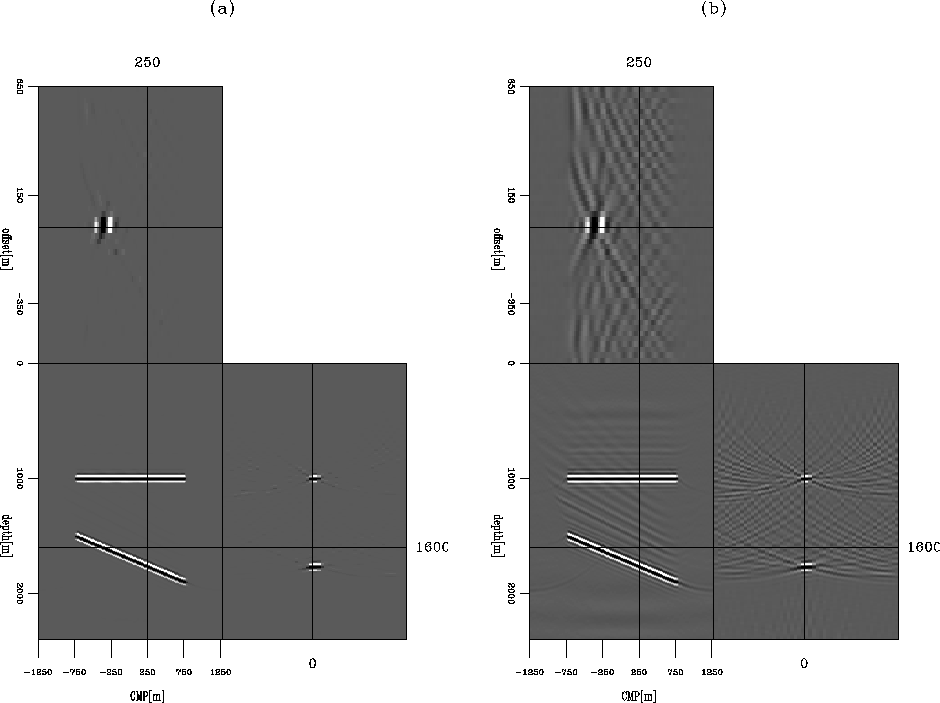
The effect is more obvious if we transform the SODCIGs into the ADCIGs, which are shown in
Figure 4; there are some gaps in the middle
of the ADCIGs (Figure 4(b)) obtained by migrating the incomplete data set,
indicating that there are some illumination problems.
of the traces in the offset dimension
with zeros. The incomplete and sparse data set is shown in Figure 2(b). Then I perform
DSR migration on both data sets to generate the SODCIGs; the corresponding migrated image cubes are shown in
Figure 3. Comparing Figure 3(a) with
Figure 3(b), we can see that even with the complete data set (Figure 2(a)),
the SODCIGs suffer from the amplitude smearing effects
caused by the offset truncation. The situation gets worse
as the offset coverage is further reduced; there are severe
amplitude smearing and aliasing artifacts in the SODCIGs as shown in Figure 3(b),
and because of the interference
of these artifacts in the offset domain, the resolution of the migrated image (i.e. offset=0) is also degraded.
The effect is more obvious if we transform the SODCIGs into the ADCIGs, which are shown in
Figure 4; there are some gaps in the middle
of the ADCIGs (Figure 4(b)) obtained by migrating the incomplete data set,
indicating that there are some illumination problems.
layer_vel
Figure 1 The velocity model for the two-layer model.
|
|  |


 layer_mod
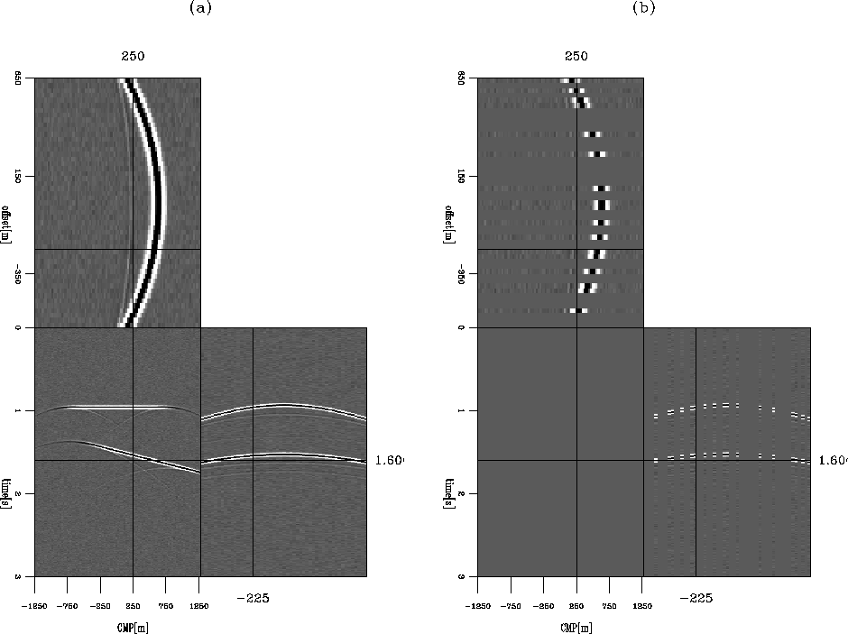
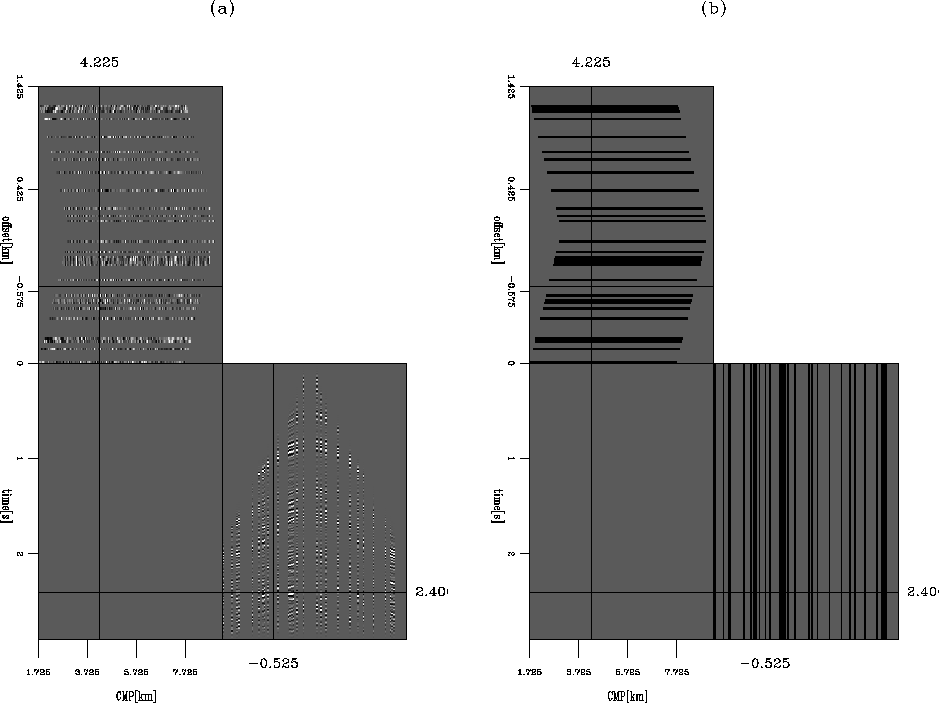
Figure 2 (a) The synthetic data set for the two-layer model,
(b) the incomplete data set with about of the traces in
the offset dimension replaced by zeros.
layer_sodcig
Figure 3 SODCIGs for the two-layer model,
(a) obtained by migrating Figure 2(a) and
(b) obtained by migrating Figure 2(b).
In both plots, the panel in the middle shows the migrated image (h=0),
the panel on the right shows the SODCIGs and the panel on the top shows the depth slice.
layer_adcig
Figure 4 ADCIGs for the two-layer model,
(a) computed from Figure 3(a), and
(b) computed from Figure 3(b).
In both plots, the panel in the middle shows the image for each opening angle,
the panel on the right shows the ADCIGs and the panel on the top shows the depth slice.
From this simple experiment, we intuitively understand that the amplitude smearing in the SODCIGs is
another representation of poor illumination and that the more energy smearing we see in the SODCIGs, the
more severe the illumination problem must be. Therefore, if we could make the energy more concentrated at zero-offset
and penalize the energy at nonzero-offset, we would compensate for
the illumination problem and fill the holes in the ADCIGs. To achieve this purpose,
I first approximate the weighted Hessian matrix
with equation (41), then solve the inversion problem based on the
fitting goals (45) and (46). The reference image  or
or  is chosen to be the migrated image
cube of the incomplete data, which is shown in Figure 2(b). The weight
is chosen to be the migrated image
cube of the incomplete data, which is shown in Figure 2(b). The weight  is
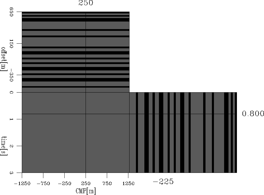
created by demigrating and then migrating the demigrated image again. The mask weight is shown in
Figure 5. As I apply the sparseness constraint along the offset dimension depth-by-depth
and CMP-by-CMP, it would be inappropriate to use a global parameter
is
created by demigrating and then migrating the demigrated image again. The mask weight is shown in
Figure 5. As I apply the sparseness constraint along the offset dimension depth-by-depth
and CMP-by-CMP, it would be inappropriate to use a global parameter  to control the sparseness; therefore
I apply locally, choosing for its value the mean value of the current offset vector. The final inversion
result is shown in Figure 6(a); for comparison, Figure 6(b)
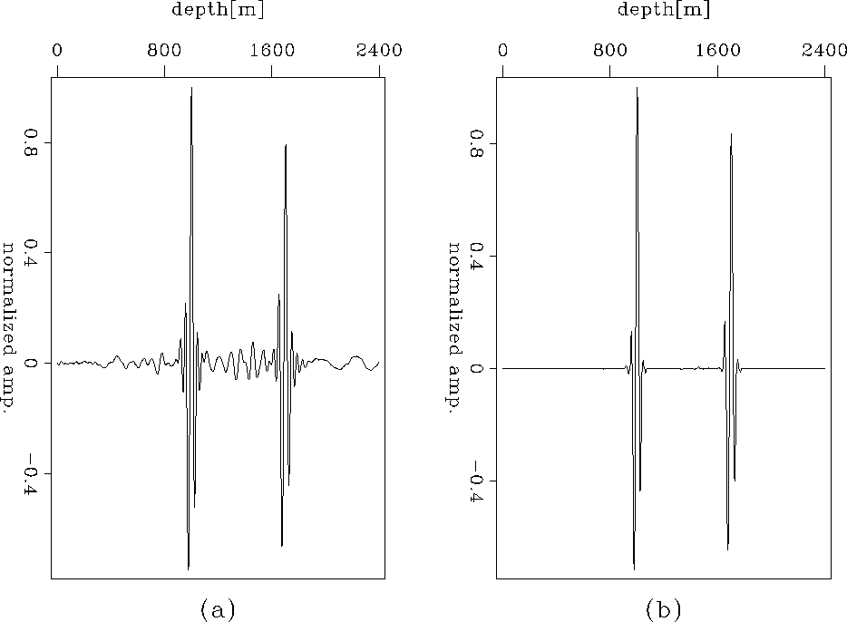
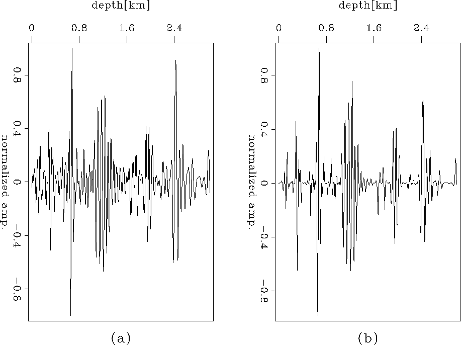
shows the migration result. Figure 7 illustrates one single
trace located at CMP= meters and offset= meters, Figure 7(a) is the result by migration,
while Figure 7(b) is
the result by inversion, where both (a) and (b) are normalized to compare their relative amplitude ratios.
From the results we can clearly see that the DSO regularization
term perfectly eliminates the energy at non-zero offset. The sparseness constraint also successfully penalizes
weak amplitudes and consequently improves the resolution of the image. Figure 8
shows the comparison of ADCIGs between migration and inversion, where, as expected, the inversion result in
Figure 8(a) fills the illumination gaps presented in Figure 8(b).
to control the sparseness; therefore
I apply locally, choosing for its value the mean value of the current offset vector. The final inversion
result is shown in Figure 6(a); for comparison, Figure 6(b)
shows the migration result. Figure 7 illustrates one single
trace located at CMP= meters and offset= meters, Figure 7(a) is the result by migration,
while Figure 7(b) is
the result by inversion, where both (a) and (b) are normalized to compare their relative amplitude ratios.
From the results we can clearly see that the DSO regularization
term perfectly eliminates the energy at non-zero offset. The sparseness constraint also successfully penalizes
weak amplitudes and consequently improves the resolution of the image. Figure 8
shows the comparison of ADCIGs between migration and inversion, where, as expected, the inversion result in
Figure 8(a) fills the illumination gaps presented in Figure 8(b).
layer_rn70_mask
Figure 5 The computed mask weight from Figure 2(b).
Black stands for ones, while grey stands for zeros.
|
|  |
layer_inv_sodcig
Figure 6 SODCIGs for the two-layer model.
(a) The inversion result, and
(b) the migration result.
Note the inversion result has perfectly penalized the energy
far from zero-offset locations and the sidelobes of the amplitudes
as well.
layer_wavelet
Figure 7 Comparison of a single trace located at CMP=0 meter and offset=0 meter.
(a) The migration result, (b) the inversion result.
The amplitudes in both (a) and (b) are normalized to compare
their relative ratios.
layer_inv_adcig
Figure 8 ADCIGs for the two-layer model.
(a) The inversion result, (b) the migration result.
Note the inversion has filled in the illumination holes.
The model with two reflectors in the previous example is simple.
To test whether the inversion scheme works for complex models, I apply it
to the Marmousi model, which is shown in Figure 9(a), again with about of the traces in
the offset dimension replaced with zeros. The computed mask weight is shown in
Figure 9(b). As before, I use the migrated image cube as the reference image cube for
computing the weighting matrices and . The parameter is also chosen to
be the mean value of the current offset vector. Because there are no good suggestions for the parameter  ,it is chosen by trial and error to get a satisfactory result. Since I use only one reference velocity
(the average between the maximum and the minimum velocities at each depth step) for
the DSR-SSF algorithm, some steeply dipping faults are not well imaged,
and because of the inaccuracy of the reference velocity,
some locations are mispositioned, indicating there should be some residual moveout in both SODCIGs and ADCIGs.
,it is chosen by trial and error to get a satisfactory result. Since I use only one reference velocity
(the average between the maximum and the minimum velocities at each depth step) for
the DSR-SSF algorithm, some steeply dipping faults are not well imaged,
and because of the inaccuracy of the reference velocity,
some locations are mispositioned, indicating there should be some residual moveout in both SODCIGs and ADCIGs.
mar_model
Figure 9 The Marmousi data set (a) and the corresponding mask weight (b),
where black stands for ones, while grey stands for zeros.
The final inversion result is shown in Figure10 (b);
for comparison, Figure10(a) is the migration result. By using the approximated inversion scheme, we
suppress the weak and incoherent noise and obtain a much cleaner result, while also improving the resulotion
to some extent. This is more obvious if we extract a single trace from the migration result and the inversion result
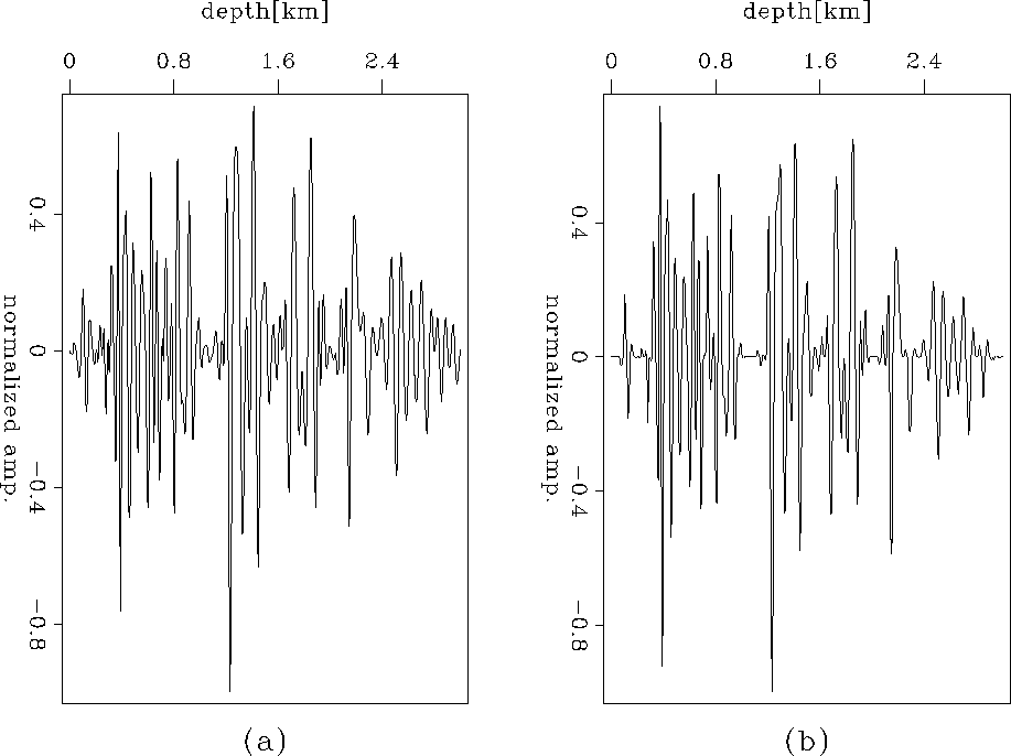
to compare their relative amplitudes. Figure 11 shows
the extracted trace located at CMP=4 km, offset= km, while Figure 12 shows
the extracted trace located at CMP=7.5 km, offset= km. In both figures, (a) is obtained from
the migration result, while (b) is obtained from the inversion result.
From Figure 11 and Figure 12, we can see that small amplitudes and the sidelobes
of the wavelets are penalized by the inversion scheme and the inversion result yields
an image with higher resolution. But also notice that some weak reflections which are presented in the migration
result are attenuated in the inversion result.
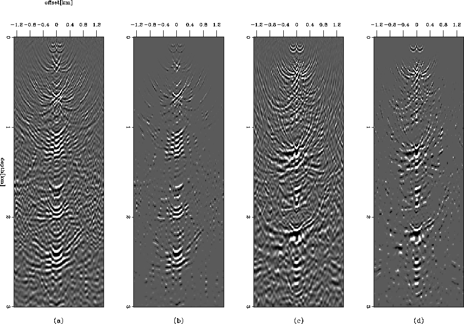
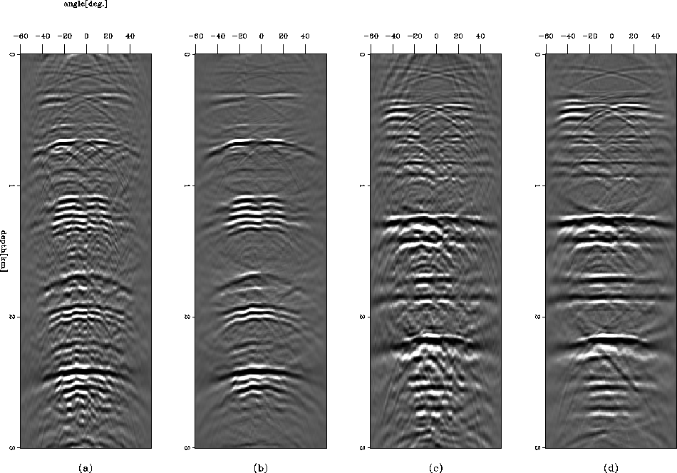
Figure 13 illustrates the SODCIGs for two different locations;
(a) and (c) are the SODCIGs at CMP=4 km and CMP=7.5 km respectively
obtained from the migration result, while (b) and (d)
show the SODCIGs at the same CMP locations obtained from the inversion result. Because of the DSO regularization
term in the inversion scheme, events that are far from zero-offset locations are penalized,
making the energy more concentrated at zero-offset. The ADCIGs at the corresponding locations shown in
Figure 14 explain this further, with the ADCIGs (Figure 14(b) and (d))
from the inversion
result smoothed across angles and the illumination holes present in (a) and (c) filled in to some degree.
As mentioned above, because of the inaccuracy of the reference velocity, there are still some residual moveouts
at some locations in both SODCIGs and ADCIGs, as seen in Figure 13(a) and Figure 14(a).
One nice thing to see is by choosing a proper trade-off parameter , the proposed inversion scheme
can successfully preserve the residual moveouts both in SODCIGs and ADCIGs,
as shown in Figure 13(b) and Figure 14(b).
The angle gathers even get cleaner, which makes it much easier to estimate
the residual moveouts. Therefore, this approximated inversion scheme may have the potential to improve the
accuracy of residual moveout estimation, and consequently improve velocity estimation results. However,
this still needs further investigation.
mar_h0
Figure 10 Comparison of the migration result and the inversion result.
(a) The image obtained by migration, and (b) the image obtained by inversion.
mar_wavelet1
Figure 11 Comparison of a single trace located at CMP=4 km and offset= km.
(a) The result from migration, and (b) the result from inversion.
The amplitudes in both (a) and (b) are normalized to compare
their relative ratios.
mar_wavelet2
Figure 12 Comparison of a single trace located at CMP=7.5 km and offset= km.
(a) The result from migration, and (b) the result from inversion.
The amplitudes in both (a) and (b) are normalized to compare
their relative ratios.
mar_sodcig
Figure 13 Subsurface-offset-domain common-image gathers for
two different surface locations.
Panels (a) and (c) are the SODCIGs at CMP=4.0 km and CMP=7.5 km obtained by migration,
while (b) and (d) are the corresponding SODCIGs obtained by inversion.
mar_adcig
Figure 14 Angle-domain common-image gathers for two different surface locations.
Panels (a) and (c) are the ADCIGs at CMP=4.0 km and CMP=7.5 km obtained by migration,
while (b) and (d) are the corresponding ADCIGs obtained by inversion.
Next: discussion and conclusion
Up: Tang: Regularized inversion
Previous: diagonal approximation of Hessian
Stanford Exploration Project
1/16/2007