Results for second model

The non-interaction approximation is not quite so simple for the second model as it was for the first. In particular, having $\nu_0 = 0.4375$for this model, we find that the NIA already gives more complicated behavior since  

$$\frac{K_0}{K_{NI}} = 1 + 11.5\rho$$ (20)

for effective bulk modulus K_NI, and  

$$\frac{G_0}{G_{NI}} = 1 + 1.168\rho$$ (21)

for effective shear modulus G_NI where K₀ = 16.86 GPa, G₀ = 2.20 GPa, and $\nu_0 = 0.4375$.So Poisson's ratio does not remain constant for this NIA model.

In the Sayers and Kachanov (1991) scheme, $\eta_1(0) = -0.01920$ GPa^-1 and $\eta_2(0) = 0.3994$ GPa^-1, as determined by the differential scheme (DS).

Without fitting

 

Fig6 Figure 6 Same as Figure 2 for a different background medium having Poisson's ratio 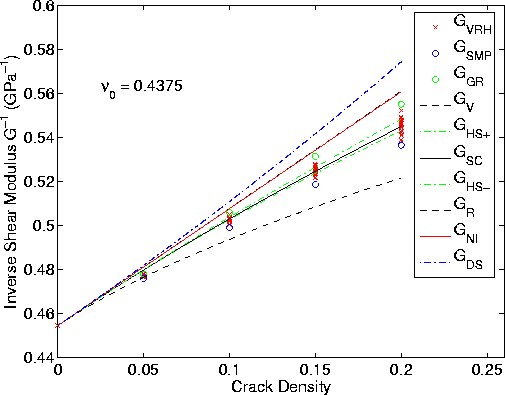$\nu_0 = 0.4375$. The estimates of individual grain behavior as crack density increases make use of $\eta_1 = - 0.0191973$ GPa-1 and $\eta_2 = 0.399406$ GPa-1 (see Sayers and Kachanov (1991) for definitions of the $\eta$'s) determined using the DS estimator for small crack densities. Similarly, for the NI estimator: $\eta_1 = - 0.0191$ GPa-1 and $\eta_2 = 0.3982$ GPa-1. Note that, again without any fitting, the estimates of inverse shear modulus are quite accurate for this model.

 

Fig7 Figure 7 Same as Figure 6 for inverse bulk modulus. Note that the estimates are again quite high for the inverse bulk modulus when compared to the numerical data. This result is in contrast to the shear modulus example in Figure 6, where the initial estimates were very close to the numerical data, both in average and spread.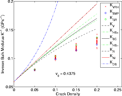

Results for the second model using only the NIA as input to the random polycrystal of cracked-grains model are displayed in Figures 6 and 7. Again, for comparison, we also show the outputs from the same set of theoretical approaches as before. Stiffness matrix data were again converted to Voigt-Reuss-Hill estimates of shear and bulk moduli for the plots. All curves converge at low crack densities, and we find the numerical data deviate from the NIA curve substantially for both shear and bulk moduli. But deviations of the numerical data from the random polycrystal method predictions are especially strong for the bulk modulus estimates. With no fitting, the shear modulus estimates have values that are centered about the self-consistent polycrystal estimates, and that lie between the Voigt and Reuss bounds. This shear modulus agreement (but without fitting) is actually better than that of the corresponding case for the first model. In contrast, the bulk modulus estimates are always significantly higher than even the Voigt upper bound (recall that the plots are inverse moduli). Again we interpret this difference between shear modulus and bulk modulus results as probably being due to the presence of longer range interactions for bulk modulus effects, and shorter range interactions for shear modulus effects. Also, the random polycrystal grain model appears to be a good model for the shear behavior, but in this case a considerably worse model for the bulk behavior -- at least until the quadratic corrections are applied.

Again, we can modify the results of the polycrystals of cracked grains model by including higher order corrections from the Sayers and Kachanov (1991) model, and do so now.

With fitting

 

Fig8 Figure 8 Same as Figure 4 for the case with 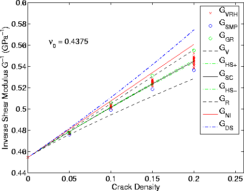$\nu_0 = 0.4375$.In this case, the spread in the data is smaller than the difference in the Reuss and Voigt bounds, but again significantly greater than that of the HS bounds.

 

Fig9 Figure 9 Same as Figure 5 for the case with 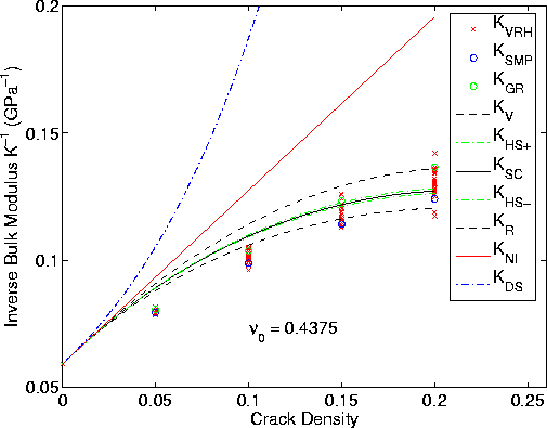$\nu_0 = 0.4375$.Spread in the inverse bulk modulus values (x) is again comparable to that between the Reuss and Voigt bounds. But some of the numerical data at $\rho = 0.05$ and $\rho = 0.10$ could not be fit for this example using the simple quadratic corrections described in the text.

Fitting the numerical data using linear, as well as quadratic, corrections to the basic Sayers and Kachanov (1991) approach, we obtain Figures 8 and 9. This second model is also more complicated than the first since it requires us to consider both diagonal and off-diagonal contributions to the compliance matrix. In particular, Figure 8 shows the bulk modulus is greatly underpredicted. But this time it is both possible and desirable to make off-diagonal corrections. The problem in doing so is that the initial shear modulus estimates are already so good that it would be preferable to make changes that do not affect the quality of the shear modulus results -- assuming that this is possible. One type of change that yields the desired behavior is a uniform change to all the coefficients having to do with the principal stresses and strains. So we might want to make changes only to S₁₁, S₂₂, S₃₃, S₁₂ = S₂₁, S₁₃ = S₃₁, and S₂₃ = S₃₂. Changing them all by the same amount will not affect the Reuss average for shear modulus, but may affect the Voigt average and the self-consistent estimate. However, we found again that $\eta_4 = 0.0$ was an appropriate value, and therefore did not make any change of this type.

Another alternative discussed previously that produces relatively small changes in shear modulus, while also changing bulk modulus, is one of the form $\Delta_{33} = 2(\eta_3 + \eta_5)\rho^2$added to S₃₃, while at the same time adding corrections $\Delta_{44} = \Delta_{55} = 2\eta_5\rho^2 = -2\Delta_{33}/3$to S₄₄ and S₅₅. This type of shift causes a very small or no change in the Reuss average for shear. By choosing $\Delta_{33} = -0.00825(\rho/0.05)^2/2$, we obtained the results observed in Figures 8 and 9. The numerical values were chosen by trial and error, based on the results observed in the plots. We chose to fit the values at the highest available values of crack density, even though this seemed to force the fit at lower crack densities to be worse than could have been achieved with other parameter values. We do not claim that our search has been exhaustive. There might be better choices to be made, and especially so if the number of $\eta$parameters included in the search were increased. The observed fit is certainly not as good for this second model as it was for the first.

Final results for the significant crack-influence parameters of both models are summarized in TABLE 1.

1.2

TABLE 1.Values of five crack-influence parameters for the two models considered.

$$0.15in] \begin{tabular} {\vert c\vert c\vert c\vert} \hline... ...pace (GPa$^{-1}$) & ~0.0917 & ~0.5500 \hline\hline\end{tabular}$$