Inversion Results

This section details the tests of the waveform inversion procedure described above on a 1D synthetic data model (left panel of figure 10). The velocity perturbation is centered at 1 km depth, is 0.2 km thick, and is $10\%$ greater than the background field of 2 kms^-1. The goal of the waveform inversion test is to reconstruct the velocity perturbation starting from an initially constant velocity model of 2 kms^-1. The true velocity profile was input to the SU finite difference modeling package Stockwell (1997), which generated data consisting of a linear direct arrival and two reflection hyperbolas of opposing sign (right panel).

 

ModelData
Figure 10 Model used for the waveform inversion test (left panel) and the data generated by FD modeling (right panel).

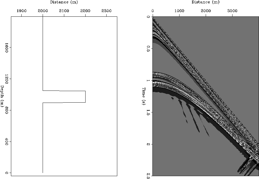
Synthetic data were subject to initial preprocessing, including low-pass filtering (high corner of 12Hz), windowing to eliminate boundary artifacts, and zeroing traces < 2 km from the source point. I applied the the latter procedure because the RWE modeling procedure cannot generate accurate wavefield data nearer to the source point. A subset of frequencies ranging from 3-12 Hz in roughly 0.25 Hz intervals were selected for inversion.

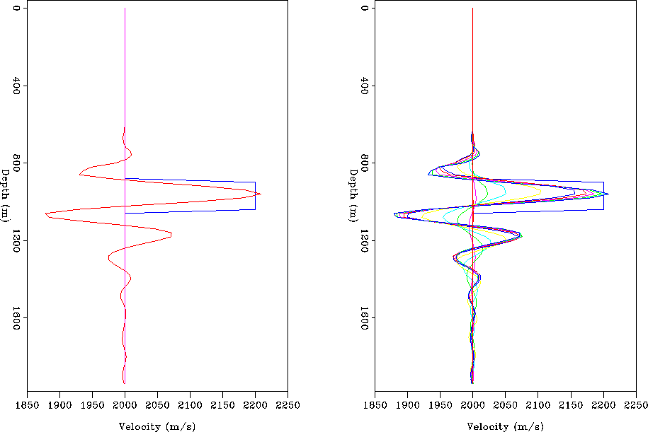
Figure 11 presents the waveform inversion results after 5 non-linear iterations. The left panel shows the final estimated perturbation, while the multiple profiles in the right panel show the cumulative velocity perturbation recovered at each integer frequency value between 3-12 Hz. The recovered velocity profile perturbation is centered almost at the correct location. Significant negative side lobes are present both above and below the true perturbation. This observation is somewhat expected because it exhibits a similar phenomenon to that noted in the 1D experimental findings of Sirgue and Pratt (2004).

 

Perturbation
Figure 11 Waveform inversion result for the model and data shown in figure 10 after 5 non-linear iterations in the 3-12 Hz frequency band. Left panel: Recovered vertical velocity profile. Right panel: Vertical velocity profile built up by each successive integer frequency.

The recovered perturbation evidently does not contain certain spatial frequency components. One way to better understand this is examining the Fourier spectra of the 1D depth profile (see figure 12). This panel shows the spatial frequency content of both the model and estimated perturbation. The recovered perturbation is lacking energy at the lower frequencies and is somewhat overestimated at mid-range. This observation suggests that the inversion does not use data with either: i) low enough temporal frequencies; or ii) sufficiently wide offsets to generate the "image-stretch" phenomena Sirgue and Pratt (2004).

 

Frequencies Figure 12 Fourier spectra of the 1D model and recovered perturbation shown in the left panel of figure  11.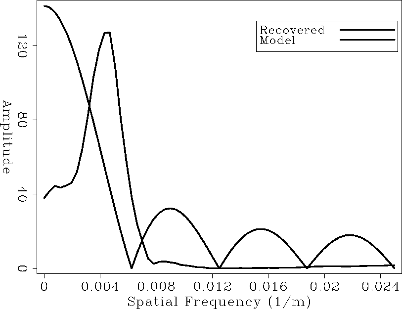

One detail important for stabilizing the inversion is to include a near-surface filter on the model space. I implement the filter as a frequency-dependent vertical mask that prevents changes to the velocity model within the first Fresnel zone of the wavepath. The masking operation is essential because it rejects stronger near-surface anomalies that lead to significant non-linear behavior and corresponding wavepath defocusing. I applied no other regularization scheme in the inversion problem solution; however, additional terms could in principle be included.