Input data precision

To understand why we can reduce the precision of our input data without meaningful loss in final image quality it is important to remember that migraton is summing along a surface in multi-dimensional space. Imagine the process of forming an image m at a given ix,iy, and iz. To form this one point in image space involves a sumation over a five-dimensional (t,h_x,h_y,m_x,m_y) input space of the data $\bf d$ multiplied by the Green's function $\bf G$, 

$$m(ix,iy,iz)= \sum_{m=1}^{ndhx} \sum_{l=1}^{ndhy} \sum_{k=... ...ndmy} \sum_{i=1}^{nt} G(i,j,k,l,m,ix,iy,iz) d(i,j,k,l,m) ,$$ (1)

where ndhx, ndhy, ndmx, ndmy, and nt are the maximum number of samples of the data in all five dimensions. In reality $\bf G$ is limited by aperature range in space and only has a few non-zero elements along the time axis, but still we are summing over a very large number of points to form a single output location.

When we reduce the precision of our data what we are really doing is introducing an error in each data sample, as a result Equation(1) becomes

 

$$m(ix,iy,iz)= \sum_{=1}^{ndhx} \sum_{j=1}^{ndhy} \sum_{k=1... ...m=1}^{nt} G(i,j,k,l,m,ix,iy,iz)( d(i,j,k,l,m)+e(i,j,k,l,m)) ,$$ (2)

where e is the error associated with reducing the data precision. When we reduce the precision we are quantizing our data. The quantization process is zero mean and has a standard deviation of $\frac{q^2}{12}$ where q is our quantization interval. $\bf G$ has relatively low amplitude variation so should not emphasize the quantization error in any coherent manner. For this analysis we can think of rewriting

Equation (2) as  

$$m(ix,iy,iz)= \sum_{i=1}^{ndhx} \sum_{j=1}^{ndhy} \sum_{k=... ...j,k,l,m,ix,iy,iz) d(i,j,k,l,m)+ G_{{\rm approx}}\sum_i^ne(i) ,$$ (3)

where n is the number of non-zero elements of $\bf G$and $G_{{\rm approx}}$ is a scalar with the mean non-zero value of $\bf G$.Most error analysis theory assumes that our errors have a normal rather than an uniform distribution, so we won't get quite the same level of error reduction, but generally the error $\bf e_{{\rm mig}}$ in our migration result by quantizing are data should be a little higher than

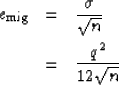$$\begin{eqnarray} e_{{\rm mig}}&=& \frac{\sigma}{\sqrt{n}} \nonumber \ &=& \frac{q^2}{12\sqrt{n}}\end{eqnarray}$$ (4)

The size of n is going to depend on what type of problem we are doing. If we want velocity information, our image space has an offset or angle axis n will be smaller and we will have to have a smaller quantization step to obtain an equivalent image.