Method

The flattening method described in Lomask et al. (2005) creates a time-shift (or depth-shift) field $\boldsymbol{\tau}(x,y,t)$ such that its gradient approximates the dip $\bf{p}\rm (x,y,\boldsymbol{\tau})$. The dip is a function of $\boldsymbol{\tau}$ because for any given horizon, the appropriate dips to be summed are the dips along the horizon itself. Using the gradient operator ($\boldsymbol\nabla=[ \frac{\partial }{\partial x} \; \; \frac{\partial }{\partial y}]^T$) and the estimated dip (${\bf p} = [{{\bf p}_x} \; \; {{\bf p}_y}]^T$), our regression is

$$\boldsymbol{\nabla} {\boldsymbol \tau}(x,y,t)\quad = \quad {\bf p}(x,y,{\boldsymbol \tau}).$$ (1)

To add regularization in the time direction, we apply a 3D gradient operator with a residual weight ${\bf W}_\epsilon$ that controls the amount of vertical regularization defined as

$${\bf W}_\epsilon\boldsymbol{\nabla}= \left[ \begin{array} {c... ... \ \frac{ \partial }{ \partial t} \end{array} \right] \quad ,$$ (2)

where ${\bf W}_\epsilon$ is a large block diagonal matrix consisting of two identity matrices $\bold I$ and a diagonal matrix $\boldsymbol{\epsilon}$=$\epsilon \bold I$.For simplicity, we implicitly chain this weight operator to the gradient operator to create a new operator now defined as a 3D gradient with an weighting parameter $\epsilon$ as  

$$\boldsymbol{\nabla}_\epsilon \quad = \quad \left[ \begin{arr... ...ilon \frac{ \partial }{ \partial t} \end{array} \right] \quad .$$ (3)

The residual is defined as  

$$\bf r \quad = \quad { \boldsymbol{\nabla}_\epsilon \boldsymb... ...}{{\bf p}_x} \ {{\bf p}_y} \ {\bf 0} \end{array} \right] }.$$ (4)

We solve this using a Gauss-Newton approach by iterating over equations (5)-(7), i.e.,

		 iterate {    

$$\begin{eqnarray} \bf r \quad &=& \quad [\boldsymbol{\nabla}_\epsilon \boldsymbol... ...bol{\boldsymbol{\tau}}_{k} + \Delta \boldsymbol{\boldsymbol{\tau}}\end{eqnarray}$$ (5) (6) (7)

		  }  ,

where the subscript k denotes the iteration number.

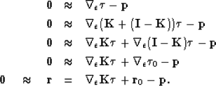
We wish to add a model mask $\bf K$ to prevent changes to specific areas of an initial $\boldsymbol{\tau}_0$ field. This initial $\boldsymbol{\tau}_0$ field can be picks from any source. In general, they may come from a manually picked horizon or group of horizons. These initial constraints do not have to be a continuous surfaces but instead could be isolated picks, such as well-to-seismic ties. To apply the mask we follow the same the development as the operator approach to missing data in Claerbout (1999) as

$$\begin{eqnarray} \bold 0 &\approx& \boldsymbol{\nabla}_\epsilon \boldsymbol{\ta... ...mbol{\nabla}_\epsilon\bold K\boldsymbol{\tau} + \bold r_0 - \bf p.\end{eqnarray}$$ (8) (9) (10) (11) (12)

Our resulting equations are now

		 iterate {    

$$\begin{eqnarray} \bf r \quad &=& \quad \boldsymbol{\nabla}_\epsilon {\bf K}\bold... ...bol{\boldsymbol{\tau}}_{k} + \Delta \boldsymbol{\boldsymbol{\tau}}\end{eqnarray}$$ (13) (14) (15)

		  }  .

Typically, we solve equation (6) in the Fourier domain, however in equation (14), $\bf K$ is non-stationary making its application in the Fourier domain difficult if not impossible. Therefore, for now we solve it in the time domain using conjugate gradients.
 

• Preconditioning with the helical derivative