Modeling of an isolated SODCIG

The modeling process starts from the prestack image $I\left(z_\xi,x_\xi,h_\xi\right)$that is function of the image-space coordinates: depth $z_\xi$, horizontal location $x_\xi$,and horizontal subsurface offset $h_\xi$.We then extract from the whole image a single SODCIG identified by its horizontal coordinate $x_\xi^{i}$,and model the corresponding aerial-shot data $D^s_{x_\xi^{i}}$and aerial-receiver data $D^g_{x_\xi^{i}}$by propagating the source wavefield $P^s_{x_\xi^{i}}$and the receiver wavefield $P^g_{x_\xi^{i}}$starting from the following initial conditions:

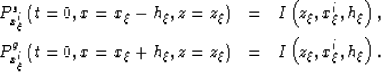$$\begin{eqnarray} P^s_{x_\xi^{i}}\left(t=0,x=x_\xi-h_\xi,z=z_\xi\right) &=& I\l... ...xi+h_\xi,z=z_\xi\right) &=& I\left(z_\xi,x_\xi^{i},h_\xi\right).\end{eqnarray}$$ (1) (2)

The receiver wavefield is propagated forward in time (t), whereas the source wavefield is propagated backward in time.

The modeled-data gathers are generated by extracting the wavefields values at the surface for all times and all surface locations as follows:

$$\begin{eqnarray} D^s_{x_\xi^{i}}\left(t,x\right) &=& P^s_{x_\xi^{i}}\left(t,x,... ...xi^{i}}\left(t,x\right) &=& P^g_{x_\xi^{i}}\left(t,x,z=0\right).\end{eqnarray}$$ (3) (4)

The simple modeling procedure illustrated above generates data useful for analyzing only flat reflectors. A generalization of this procedure to reflectors with arbitrary dips can be simply achieved by tilting the source function and aligning it along the normal to the reflector instead of along the vertical; that is, by interpreting the offset as the geological-dip offset instead of as the horizontal offset. Biondi and Symes (2004) provide a kinematic analysis of SODCIGs from dipping reflectors that justify the following generalization of equations 1 and 2:

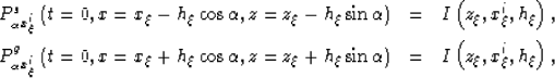$$\begin{eqnarray} P^s_{_{\alpha}x_\xi^{i}}\left(t=0,x=x_\xi-h_\xi\cos\alpha,z=z_\... ...+h_\xi\sin\alpha\right) &=& I\left(z_\xi,x_\xi^{i},h_\xi\right),\end{eqnarray}$$ (5) (6)

and correspondingly,

$$\begin{eqnarray} D^s_{_{\alpha}x_\xi^{i}}\left(t,x\right) &=& P^s_{_{\alpha}x_... ...eft(t,x\right) &=& P^g_{_{\alpha}x_\xi^{i}}\left(t,x,z=0\right).\end{eqnarray}$$ (7) (8)

To illustrate the proposed modeling procedure I applied it to a SODCIG extracted from the prestack image of a simple synthetic data set. The data were modeled by using the two-way wave equation and by assuming a constant propagation velocity of 1 km/s and two reflectors: a flat reflector below a reflector dipping by 10 degrees. The complete data set comprises a total of 100 split-spread shot gathers. I migrated the data twice by source-receiver migration: once using the correct velocity and once using a velocity too slow by 10%. Figure , shows the zero-subsurface-offset sections obtained by migration with the correct velocity (Figure a), and a velocity too slow by 10% (Figure b).

 

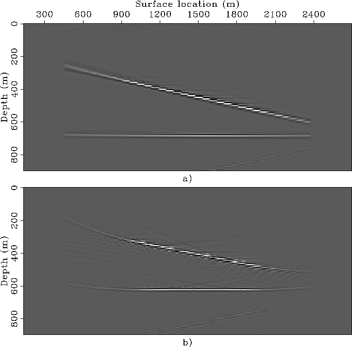
Sections-overn Figure 1 Zero-subsurface-offset sections obtained by source-receiver migration: a) with the correct velocity, and b) a velocity too slow by 10%.

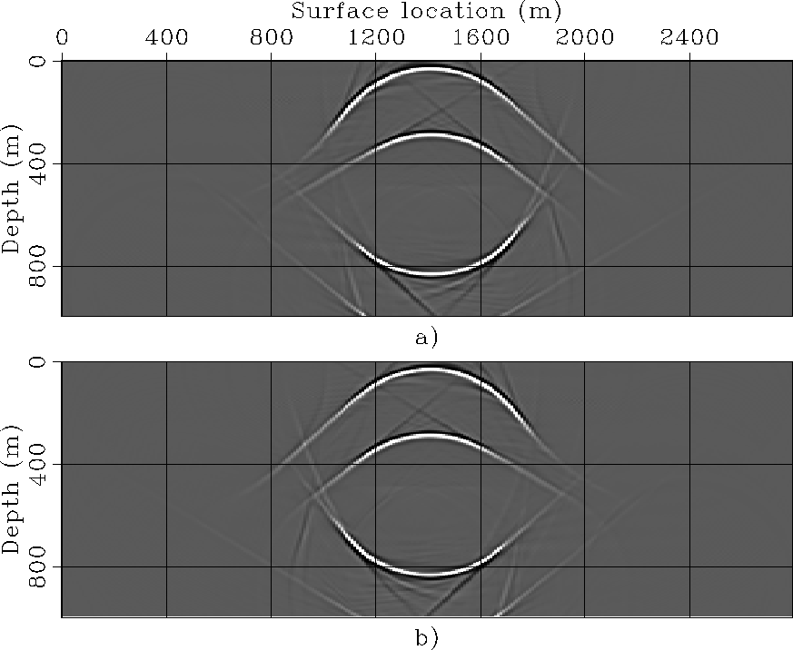
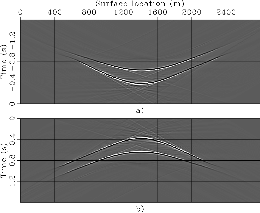
Figure  shows snapshots of the wavefields obtained by extracting an individual SODCIG from the prestack image obtained using the correct velocity (Figure a). Panel a) shows the source wavefield and panel b) shows the receiver wavefield. Figure  shows the data recorded at the surface by the aerial arrays corresponding to the wavefields shown in Figure . Notice that the source wavefield (panel a) is recorded at negative times, because it is propagated back in time. 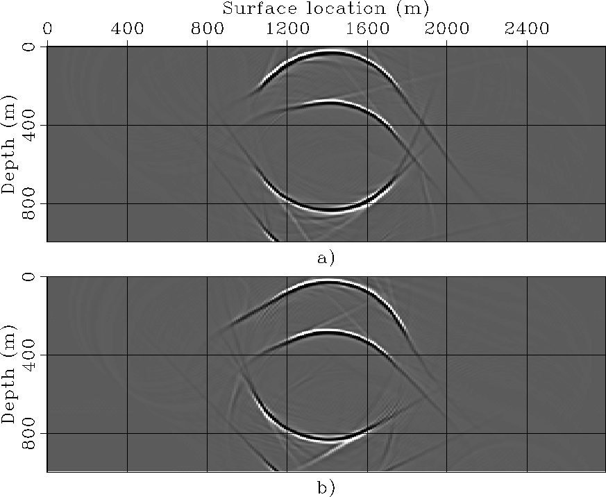Figures - shows wavefields snapshots and the recorded data corresponding to the same SODCIG used to model the data shown in Figure , but assuming the reflectors to be dipping by 45 degrees, and imposing the initial conditions expressed in equations 5 and 6. Notice that, because of the assumed reflector dip, the wavefields shown in Figure  are more asymmetric than the the wavefields shown in Figure , with the receiver wavefield (Figure b) tilted towards the right more than the source wavefield (Figure a).

 

Snaps-INF-overn Figure 2 Snapshots of the source wavefield (panel a) and the receiver wavefield (panel b) generated by modeling an isolated SODCIG by imposing the initial conditions expressed in equations 1 and 2.

 

Data-INF-overn Figure 3 The data recorded at the surface by aerial arrays and corresponding to the source wavefield (panel a) and the receiver wavefield (panel b) shown in Figure .

 

Snaps-INF-DIP-overn Figure 4 Snapshots of the source wavefield (panel a) and the receiver wavefield (panel b) generated by modeling an isolated SODCIG by imposing the initial conditions expressed in equations 5 and 6 and assuming a reflector dip of 45 degrees.

 

Data-INF-DIP-overn Figure 5 The data recorded at the surface by aerial arrays and corresponding to the source wavefield (panel a) and the receiver wavefield (panel b) shown in Figure .