


| |
(114) |
| |
(115) |
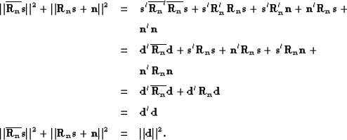
![[*]](http://sepwww.stanford.edu/latex2html/cross_ref_motif.gif) ) and
(), we have for the data vector d the following equalities:
) and
(), we have for the data vector d the following equalities:
| |
||
| (116) |
|
geom11
Figure 1 A geometric interpretation of the noise filter when n and s are not orthogonal. | 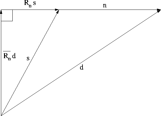 |

|
geom21
Figure 2 A geometric interpretation of the noise filter when n and s are orthogonal. | 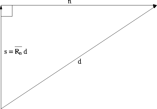 |
| |
||
| (117) |
 |
||
| (118) | ||
) and (),
the last two equalities can be written as follows:
| |
||
| (119) |
;
similarly, ). Similarly, n is in the
null space of