FEAVA detection

In order to remove FEAVO/FEAVA, or at least not to trust the amplitudes from the affected areas, one must be alerted to its existence. Visual inspection of zero-offset data for subvertical streaks of high energy provides a cue only in the case of the most powerful effects. ``Kjartansson V's'' would provide a good diagnostic tool if it were not for today's prestack data volumes which size in the terrabytes. Comparing stacks of near and far offsets is a good way of alerting that something is wrong Hatchell (2000a), but it does not highlight FEAVO specifically. Laurain et al. (2004) give a good way of quantitatively estimating the amplitudes due solely to propagation effects for a single reflector at a time. This method is even more labor-intensive than visually examining the prestack lines for ``V''s. The worst one is to rely on the interpreter to realize if ``something is wrong with the AVO'' - he may just interpolate an intercept and gradient through the erratic values. What is needed is a quick, simple and robust way to signal the corruption of AVO by focusing.

Vlad (2004b) provides such a FEAVA detection method. The method is based on the fact that reflector-caused AVA for incidence angles $\theta<30^\circ$ is very well described Shuey (1985) by  

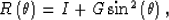$$R\left(\theta\right)=I+G\sin^2\left(\theta\right),$$ (3)

where I and G depend only on the lithology at the reflector. If the amplitudes are picked at a single midpoint-depth location not affected by focusing and plotted as a function of the $\sin^2(\theta)$,the values will arrange close to a line with intercept I and gradient G. The presence of FEAVO causes the linear dependence to break, as exemplified on a simple synthetic in Figure .

 

examine_FEAVO
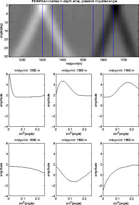
Figure 10 Top panel: Midpoint-angle depth slice from the prestack migrated synthetic dataset shown in Figure . From Vlad et al. (2003a). Bottom panels: Amplitudes at midpoints marked by vertical thin lines in the upper panel. From Vlad (2004b).

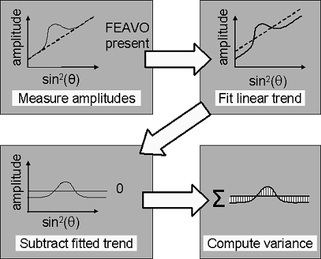
A direct estimate of the amount of FEAVA energy present at a (midpoint, depth) location can be obtained by measuring how much nonlinearity is in the dependence between amplitudes and $\sin^2(\theta)$. Simply interpolating a linear trend, subtracting it and computing the variance of the residual (Figure ) provides a computationally cheap procedure with no knobs to turn.

 

detect Figure 11 FEAVA detection flowchart. From Vlad and Biondi (2004).

The ``FEAVO attribute'' output by this detector is ``poststack-sized'', having no offset dimensions and no intensive human labor requirement for the visual examination. The vertical clustering of the affected areas in clusters under the source anomalies helps with the detection and possibly with the interpretation of the heterogeneities that cause FEAVA as well. Figure shows a simple example obtained by migrating with the background velocity the synthetic dataset from Figure .

 

anoloc Figure 12 FEAVO anomalies flagged in the midpoint-depth space by the automatic detection procedure. The stars denote the location of the heterogeneities causing the focusing. From Vlad (2004b).

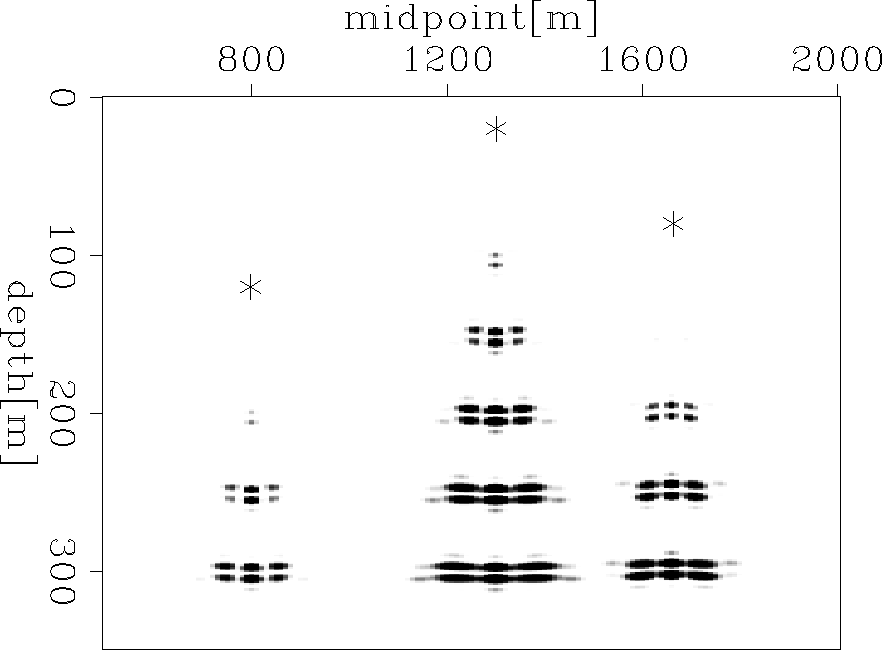The FEAVO effects are very visible - everything that is certainly not FEAVO has been eliminated. By contrast, when looking for vertical streaks or Kjartansson ``V''s in the data without the help of the detector, the eye is distracted by the very large amount of amplitudes that cannot possibly be FEAVO, but are still in the picture. Figure shows that the FEAVO detector functions well in a complex case, with subtle (2-3% variation from the background) velocity ``lenses'' which produce barely visible subvertical high amplitude streaks in the stack.

 

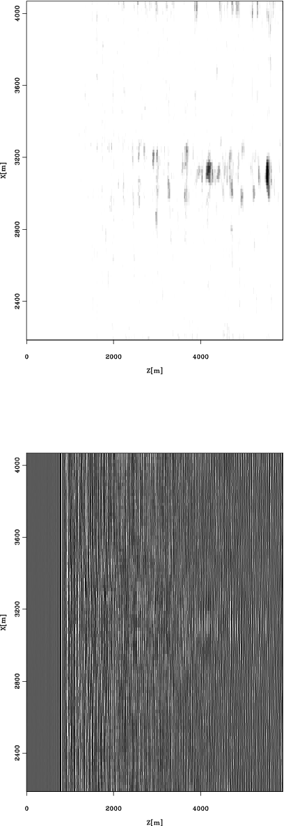
com_nomult_imag Figure 13 The FEAVO detector performs well on realistic data. Notice how barely visible focusing in the stack (top panel) is amplified by the detector (bottom panel). The erratic values in the upper part of the detector output are from above the sea bottom. From Vlad (2004a).

The robustness of the FEAVO detector is confirmed by its behavior in the presence of multiples. In Figure multiples are also weakly highlighted, but they are not vertically correlated like FEAVO and therefore they are not a serious source of noise.

The output of the detector could be improved in principle by subtracting an interpretation-based estimation of the lithology-caused AVO, instead of just the best fitting line. However, this would introduce complexity, expense and sources of errors for marginal gains. Simple as it is, the FEAVO detector works well independently for each midpoint, even when the rock-caused AVO is unknown, and even in the presence of multiples or limited aperture angles Vlad (2004a). A significant increase in complexity appears to be necessary, however, when trying to remove FEAVO from the data, which is the subject of the next section.

 

bg-refvel1top2
Figure 14 Left: V(z) migration of FEAVO-affected data with internal multiples. The streak of energy in the center is barely visible. Right: Applying the FEAVO detector really highlights the focusing effects. From Vlad (2004a).