


 |
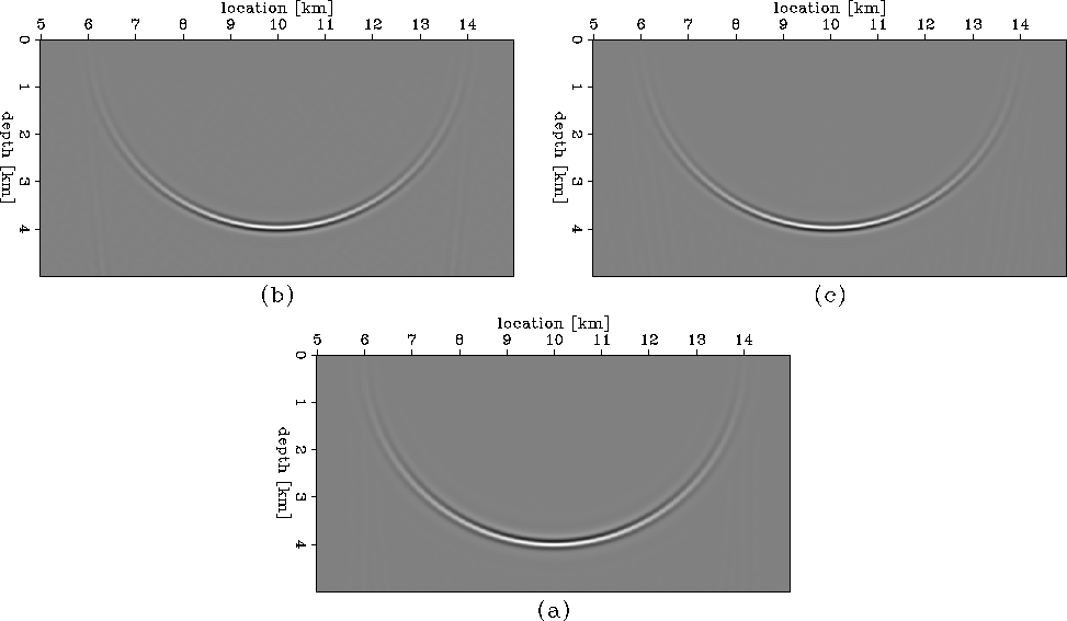
I illustrate the WEMVA method with a simple model depicted in
WEP1.imag.
The velocity is constant and the data are represented by an
impulse in space and time.
I consider two slowness models: one regarded as
the correct slowness s, and the other as
the background slowness ![]() . The two slownesses are
related by a scale factor
. The two slownesses are
related by a scale factor ![]() .For this example, I consider
.For this example, I consider ![]() to ensure that
I do not violate the requirements imposed by the Born
approximation.
to ensure that
I do not violate the requirements imposed by the Born
approximation.
Next, I migrate the data with the background slowness ![]() and store the extrapolated wavefield at all depth levels.
WEP1.imaga shows the image corresponding
to the background slowness
and store the extrapolated wavefield at all depth levels.
WEP1.imaga shows the image corresponding
to the background slowness ![]() .I also migrate the data with the correct slowness and obtain
a second image
.I also migrate the data with the correct slowness and obtain
a second image ![]() . A simple subtraction of the two images
gives the image perturbation in WEP1.imagb.
. A simple subtraction of the two images
gives the image perturbation in WEP1.imagb.
Finally, I compute an image perturbation by a simple application
of the forward WEMVA operator defined in WEMVAobj to the slowness
perturbation ![]() (WEP1.imagc).
Since the slowness perturbation is very small, the requirements
imposed by the Born approximation are fulfilled, and the
two images in WEP1.imagb and WEP1.imagc
are identical.
The image perturbations are phase-shifted by
(WEP1.imagc).
Since the slowness perturbation is very small, the requirements
imposed by the Born approximation are fulfilled, and the
two images in WEP1.imagb and WEP1.imagc
are identical.
The image perturbations are phase-shifted by ![]() relative
to the background image.
relative
to the background image.
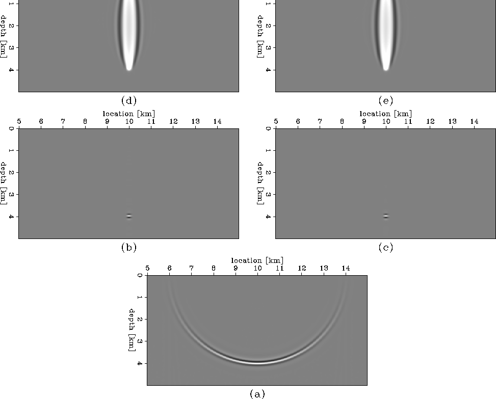
A simple illustration of the adjoint operator ![]() defined in
WEMVAobj is depicted in WEP1.rays.
Panel (a) shows the background image,
panels (b) and (c) show image perturbations, and
panels (d) and (e) show slowness perturbations.
I extract a small subset of each
image perturbation to create the impulsive image perturbations
in WEP1.raysb and WEP1.raysc.
The left panels (b and d) correspond to the image perturbation
computed as an image difference, while the panels on the right
(c and e) correspond to the image perturbation computed with the
forward WEMVA operator.
In this way, the data corresponds to a single point
on the surface, and the image perturbation corresponds to a single
point in the subsurface. By backprojecting the image perturbations
in WEP1.raysb and WEP1.raysc
with the adjoint WEMVA operator, I obtain identical
wavepaths or ``fat rays'' shown
in WEP1.raysd and WEP1.rayse,
respectively.
defined in
WEMVAobj is depicted in WEP1.rays.
Panel (a) shows the background image,
panels (b) and (c) show image perturbations, and
panels (d) and (e) show slowness perturbations.
I extract a small subset of each
image perturbation to create the impulsive image perturbations
in WEP1.raysb and WEP1.raysc.
The left panels (b and d) correspond to the image perturbation
computed as an image difference, while the panels on the right
(c and e) correspond to the image perturbation computed with the
forward WEMVA operator.
In this way, the data corresponds to a single point
on the surface, and the image perturbation corresponds to a single
point in the subsurface. By backprojecting the image perturbations
in WEP1.raysb and WEP1.raysc
with the adjoint WEMVA operator, I obtain identical
wavepaths or ``fat rays'' shown
in WEP1.raysd and WEP1.rayse,
respectively.
 |
Prestack Stolt Residual Migration (storm)
can be used to create image perturbations.
Given an image migrated with the background velocity,
I can construct another image
by using an operator ![]() function of a parameter
function of a parameter
![]() which represents the ratio of the original and modified
velocities.
The improved velocity map is unknown explicitly, although it
is described indirectly by the ratio map of the two velocities:
which represents the ratio of the original and modified
velocities.
The improved velocity map is unknown explicitly, although it
is described indirectly by the ratio map of the two velocities:
| |
(67) |
The simplest form of an image perturbation can be constructed
as a difference between an improved image (![]() ) and
the background image (
) and
the background image (![]() ):
):
| (68) |
A simple illustration of this problem is depicted in
WEP2.imag and WEP2.rays.
This example is similar with the one in
WEP1.imag and WEP1.rays, except
that the velocity ratio linking the two slownesses is much
larger: ![]() .In this case, the background and correct images are not at all
in phase, and when I subtract them I obtain two distinct events,
as shown in WEP2.imagb. In contrast,
the image perturbation obtained by the forward WEMVA operator,
WEP2.imagc, shows only one event as in the previous
example. The only difference between the image perturbations in
WEP1.imagc and WEP2.imagc is a scale
factor related to the magnitude of the slowness anomaly.
.In this case, the background and correct images are not at all
in phase, and when I subtract them I obtain two distinct events,
as shown in WEP2.imagb. In contrast,
the image perturbation obtained by the forward WEMVA operator,
WEP2.imagc, shows only one event as in the previous
example. The only difference between the image perturbations in
WEP1.imagc and WEP2.imagc is a scale
factor related to the magnitude of the slowness anomaly.
WEP2.rays depicts fat rays for each kind of image perturbation: on the left, the image perturbations obtained by subtraction of the two images, and on the right, the image perturbation obtained with the forward WEMVA operator. The fat rays corresponding to the ideal image perturbation (panels c and e) do not change from the previous example, except for a scale factor. However, in case we use image differences (panels b and d), we can violate the requirements of the Born approximation. In this case, we see slowness backprojections of opposite sign relative to the true anomaly, and also the two characteristic migration ellipsoidal side-events indicating cycle-skipping (114).


