Methodology

In Lomask and Claerbout (2002), we found that we could integrate local dip information (${\bf p}_x$) into total time shifts (${\bf t}_x=t(x)$) quickly in the Fourier domain with:

$${\bf t}_x \quad \approx \quad {\rm FFT_{\rm 1D}}^{-1} \left[... ...\nabla'{\bf p}_x \right]}\ \over { -Z_x^{-1} +2 -Z_x} \right] ,$$ (1)

where $Z_x = e^{i w \Delta x}$.

We also found that if we initialized the dips in the y direction (${\bf p}_y$) to zero, then this equation would apply some kind of regularization in the y direction:  

$${\bf t} \quad \approx \quad {\rm FFT_{\rm 2D}}^{-1} \left[{\... ...} \right]}\ \over { -Z_x^{-1} -Z_y^{-1} +4 -Z_x -Z_y} \right] ,$$ (2)

where ${\bf t}=t(x,y)$, ${\bf p} = ({\bf p}_x,{\bf p}_y)$, $Z_x = e^{i w \Delta x}$and$\ Z_y = e^{i w \Delta y}$.This would cause the integration to be smooth in the y direction. However, we were not able to control how smooth it would be.

Here we will add an adjustable regularization parameter ($\epsilon$) to equation (2). We begin with the fitting goal:

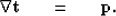$$\begin{eqnarray} \bf {\nabla t \quad }& = & \bf{ \quad p}.\end{eqnarray}$$ (3)

We can minimize the difference between the estimated slope and the theoretical slope with:

$$\begin{eqnarray} 0 \quad \approx \quad \bf {\nabla t }& - & \bf{ p}.\end{eqnarray}$$ (4)

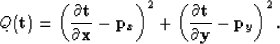
Next, we write the quadratic form to be minimized as:

$$Q(\bold t) = (\bold \nabla \bold t - \bold p)' (\bold \nabla \bold t - \bold p).$$ (5)

Because the gradient is ($\nabla=( \frac{\partial }{\partial x}, \frac{\partial }{\partial y})$), we can write:

$$Q(\bold t) = \quad \left[ \begin{array} {c} \frac{\bf \parti... ...{\bf \partial t}{\bf \partial y}-{\bf p}_y \end{array} \right].$$ (6)

This can be rewritten as:  

$$Q(\bold t) = \left( \frac{\bf \partial t}{\bf \partial x}-{\... ...eft( \frac{\bf \partial t}{\bf \partial y}-{\bf p}_y \right)^2.$$ (7)

The second term in equation (7) is the regularization term and only needs a scalar parameter $\epsilon$ to adjust its weight relative to the first term. Now we have:

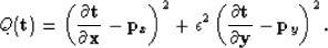$$Q(\bold t) = \left( \frac{\bf \partial t}{\bf \partial x}-{\... ...ft( \frac{\bf \partial t}{\bf \partial y}-{\bf p}_y \right)^2 .$$ (8)

Working backwards we see that it is now necessary to define a gradient operator that has an epsilon weight applied to one direction as:

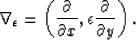$$\nabla_{\epsilon}=\left( \frac{\partial }{\partial x}, \epsilon \frac{\partial }{\partial y}\right).$$ (9)

It is also necessary to apply the scalar to the dip in the y direction as:

$${\bf p}_\epsilon=( {\bf p}_x,\epsilon {\bf p}_y).$$ (10)

Lastly, the y components of the z-transform in the denominator of equation (2) also need to be scaled. The final analytical solution with an adjustable regularization parameter is:  

$${\bf t} \quad \approx \quad {\rm FFT_{\rm 2D}}^{-1} \left[{\... ...1} -\epsilon Z_y^{-1} +2+2\epsilon -Z_x -\epsilon Z_y} \right],$$ (11)

where $Z_x = e^{i w \Delta x}$and$\ Z_y = e^{i w \Delta y}$.