Application to seismic data

To apply this segmentation method to seismic data, the weight calculation needs to be modified. Rather than looking for clusters of pixels with similar intensity, we are now looking for groups of pixels on each side of the bright amplitude salt boundary. Therefore, we want the weights connecting pixels on either side of the salt boundary to be low and the weights connecting pixels on the same side of the salt boundary to be relatively high. We get the best results when the weight for every pair of pixels is made weak(set to zero) when the following two criteria are met, otherwise the weight is made strong(set to one). The first criteria is that the minimum negative instantaneous amplitude along the shortest path between pixels is below a threshold. The threshold in our examples thus far is 85 percent of the maximum negative amplitude. The second criteria is the minimum is less than the two pixels themselves. The second criteria insures that the minimum is actually located between the two pixels. This is illustrated in Figure 1.

 

pixel Figure 1 A cartoon illustrating some sample weights on the negative instantaneous amplitude. Several pixels are shown in squares and their corresponding weights in circles. The salt boundary is defined as areas where the negative instantaneous amplitude is below a threshold.

 

amp.wt
Figure 2 Top is negative absolute value of the complex trace of a synthetic salt boundary. Bottom is the weight connecting each pixel with the pixel directly above it. It is zero where two pixels are separated by the salt boundary.

The top panel of Figure 2 shows the negative of the instantaneous amplitude of a synthetic salt boundary. This is the input for the weight calculation. The resulting weight matrix is extremely large: $({\tt m} \times {\tt n})^{\tt 2}$ where m and n are the dimensions of the image. Because this matrix is so large, checking the quality of weights is problematic. We can however view all of the weights for particular pairs of pixels. For instance, the bottom of Figure 2 is the weight between each pixel and the adjoining pixel directly above it. Notice that it follows the peak of the amplitude.

 

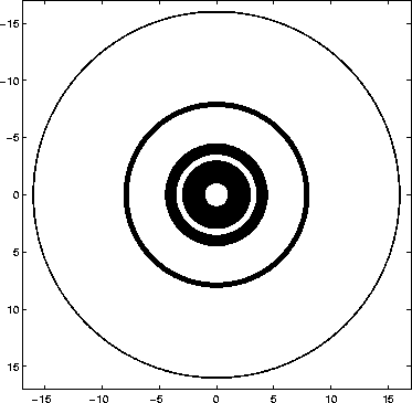
sampling Figure 3 A cartoon of the $\log_2$ sampling of one pixel up to 16 samples. The black areas are sampled.

We found that the best results are obtained when the maximum search distance is greater than 30 pixels. The maximum search distance is the maximum distance between pixels, beyond which the weights are set to zero. Using large search distances causes two problems. First, the matrix becomes more dense and requires more storage space. Second, the weights of the pixels at greater distances far outnumber those at close distances causing a bias in the weight matrix. Shi and Malik (2000) used a decaying distance weight to reduce this bias. We found that if we only use windows that are centered at powers of 2, then the matrix is still sufficiently sparse while still benefiting from greater search distances. However, this obviously causes many distances to be not sampled at all. Figure 3 shows the $\log_2$ sampling of one pixel up to a distance of 16 samples. To correct this, we plan to randomly sample from within the maximum search distance so that the number of non-zero points is approximately the same for all distances.

 

• Iterative Velocity Analysis