Application to field data

We applied the shot-profile migration methodology outlined above to a 2-D multi-offset GPR data set collected near Langley, British Columbia, Canada. The geology of the field site consists of a sand and gravel glacial outwash deposit underlain by a conductive marine clay, the depth of which varies from near surface to approximately 10 m across the profile. The data were collected along a road using a PulseEkko 100 GPR system with 100 MHz antennas oriented perpendicular to the survey line. A shot-profile survey configuration was used with 30 receiver offsets ranging from 0.5 m to 15 m, with a step size of 0.5 m. The transmitter spacing along the line was also 0.5 m, with a total of 200 shot gathers making up the approximately 100 m long profile.

Pre-processing of the Langley data included residual median filtering to remove the low frequency inductive response upon which the radar reflection signal was superimposed, and correction for drift in the zero time of the GPR instrument, most likely due to temperature fluctuations. Because the road surface was very flat, no topographic correction was needed. A time-varying exponential gain was also applied to the data to compensate for energy losses incurred by the GPR pulse during propagation.

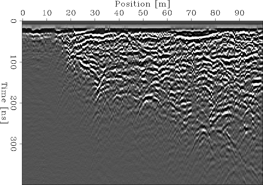
Figure (1) shows the unmigrated, near-offset (0.5 m) time section extracted from the Langley data set. This is what would be recorded in a typical, constant-offset GPR survey. Notice that the section is quite complicated, with numerous diffraction hyperbolae present and very few laterally continuous reflectors. The dipping boundary between the sand/gravel and clay layers can been seen as the region where the radar signal rapidly attenuates. However, due to the numerous diffraction hyperbolae and conflicting dips present in the section, the exact location of this boundary is difficult to determine.

In order to perform shot-profile migration, a subsurface velocity model was required. To obtain this model, the radar data were sorted into common-midpoint (CMP) gathers, and semblance analysis was performed. After picking the maximum points on the semblance scans, the resulting root-mean-square (RMS) velocity model was interpolated and converted into a map of interval velocity. The resulting model that was used for the migration is approximately v(z), with the boundary between the vadose (high-velocity) and saturated (low-velocity) zones at approximately 4.5 m.

Figure (2) shows the Langley multi-offset data after shot-profile migration.

 

time
Figure 1 Nearest-offset time section from the Langley multi-offset data set.

 

depth
Figure 2 Corresponding depth image after shot-profile migration, and a number of representative ADCIGs.

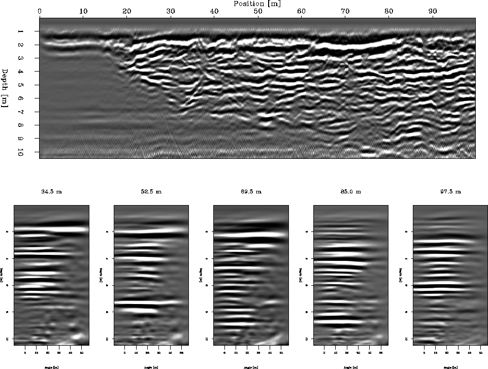As outlined in the previous section, each shot-gather was migrated through independent extrapolation of the source and receiver wavefields, and application of the imaging condition. The migrated shot gathers were then summed to produce the image shown. Also displayed in Figure (2) are a number of representative ADCIGs from the migrated data. Finite length acquisition leads to a decrease in available incidence angles for reflectors at increasing depth. For this reason, the ADCIGs become less coherent at large angle deeper in the section.

Comparing Figures (1) and (2), notice that the original time section has been significantly improved after shot-profile migration of the multi-offset data. The migrated image is much cleaner, as diffraction hyperbolas have been largely collapsed and conflicting dips due to the interference of diffraction tails have been eliminated. Many laterally continuous reflections which are absent on the time section can now been seen. Most notable is the water table, which is now very visible at approximately 4.5 m depth. Also, the boundary between the sand/gravel and clay layers is easily identified on the migrated section. On-lap of reflectors in the sand and gravel layer with this boundary can also be seen. Finally, notice that the ADCIG panels shown are very flat. This indicates that we have used an appropriate velocity model to image the data. Any remaining curvature in these gathers could be used to further refine this velocity model.