The chicken and the egg

The 2-D phase-ray extrapolation approach detailed above is analogous to the fabled 'chicken and egg' conundrum: which to compute first? Stated explicitly, phase-rays must be calculated from a known wavefield solution; however, the wavefield is itself the quantity being computed. Because the wavefield is not known a priori, clearly a new strategy is required to resolve these disparate observations.

There are (at least) two possible ways to circumvent this issue. The first procedure involves using precomputed wavefields to train the phase-ray coordinate system by: i) establishing the longer wavelength rayfield structure by raytracing in a background velocity model using a broadband solver; ii) calculating an initial monochromatic wavefield solution using the background rayfield as the coordinate system; iii) computing an updated ray-coordinate system from the previous wavefield solution; and iv) calculating an updated wavefield on the improved phase-ray coordinate system. This procedure is addressed in companion paper Shragge and Biondi (2004) in this report.

A second approach is to use wavefields parameterized in phase-ray coordinates, rather than Cartesian, to dictate the direction of the next rayfront step. For judiciously chosen $\Delta \t$ steps, both the rayfield direction and resulting wavefield evolves slowly, and ray directions differ by only small, incremental amounts in a neighborhood of $\t$. Hence, the orientation of previous few ray steps provide a good estimate of the required ray direction at the present $\t$ step. Thus, a phase-ray coordinate system may be computed on the fly using the magnitude of the wavefield phase gradient of the previous few steps and the local velocity function.

Using a wavefield parameterized in ray-coordinates to generate the underlying coordinate system requires that the governing phase-ray equations are transformed accordingly. Fortunately, the magnitude of a scalar field gradient remains invariant to coordinate transformation, and is related through a change of variables,  

$$\frac{\partial\phi}{\partial x_l} = \frac{\partial\phi}{\partial y_m}\frac{\partial y_m}{\partial x_l},$$ (11)

where x_l=[x,z] and $y_m=[\t, \gamma]$ are the Cartesian and ray coordinate basis, respectively, and l and m are dummy indices. This reparameterization leads to the ray-coordinate phase-ray equations,  

$$\frac{{\rm d}r_i}{{\rm d}s} = \frac{\partial \phi}{\partial ... ...rac{\partial y_m}{\partial x_l}\right) \right]^{-\frac{1}{2}}.$$ (12)

Equations (11) can be written explictly in Cartesian and ray variables,

$$\left[\begin{array}[pos] {c} \frac{\partial \phi}{\partial x... ...mma}\frac{\partial \gamma}{\partial z} \\ \end{array}\right].$$ (13)

The partial derivatives between the two coordinate systems in equations (11) are directly related to traditional ray parameters. Cartesian derivatives of $\t$ are the horizontal and vertical plane-wave slownesses, while those with respect to $\gamma$ are the local rotation angle to the Cartesian coordinate system (illustrated in Figure 1). Explicitly, these functions are,

$$\begin{eqnarray} \frac{\partial\t}{\partial x} = \frac{ {\rm sin}\, \theta }{v({... ...frac{\partial\gamma}{\partial z} = {\rm sin}\, \theta, \nonumber \end{eqnarray}$$ (14)

where parameter $\theta$ is the angle formed between a ray and the z-axis (assumed to be positive downward).

Computing a weighted average direction from the previous M steps requires saving M+1 previous wavefield steps. The discrete version of equation (12) for ray step at index t, $\Delta r_i^{t}$, is,

$$\Delta r_i^{t} \approx v(r_i({\bf x})) \, \Delta \t \, \sum_{m=1}^{M} \beta_m \, \, \frac{\Delta r_i^{t-m}}{\Delta s^{t-m}},$$ (15)

where $\Delta s^{t}$ is the scalar step magnitude at step t, and $\beta_m$ are a set of weights subject to,

$$\sum_{m=1}^M \beta_m = 1.$$ (16)

Weights $\beta_m$ may be chosen to yield a spline fit of at least second-order accuracy.

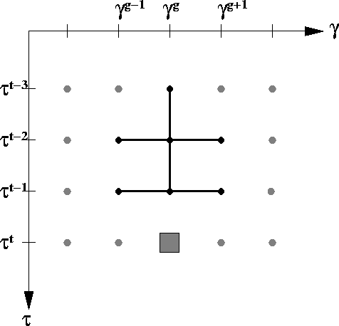
The use of previous wavefield solutions to compute solutions to equations (12) naturally gives rise to a broadened finite difference stencil. Figure 2 presents the finite difference stencil for the M=2 case that has second-order accuracy in $\gamma$ and $\t$.

 

stencil Figure 2 Finite difference stencil for calculating wavefield solution at present step using the previous two steps (M=2). The solid square represents the location of the desired rayfield solution, and the in-filled circles connected by lines are the points contributing to the solution point.