Squirt a_ij Coefficients

To obtain the a_ij coefficients in the squirt model, we first note that these coefficients are defined under conditions where $\dot{\zeta}_{\rm int}=0$ (no fluid passing between the porous grains and the principal porespace). Under these conditions, the rate of fluid depletion $\nabla \cdot {\bf q}_1$ of a sample (rate of fluid volume being extruded from the principal pore space via the exterior sample surface as normalized by the sample volume) is due to the difference between the rate of dilatation of the principal porespace (denoted here as $\dot{e}_1$) and the rate at which fluid in the pores is dilating $-\dot{\overline{p}}_{f1}/K_f$. 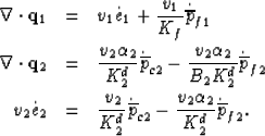If we also perform a volume average of equation (3) over the porous grain space and use the notation that $v_2 \dot{e}_2 = \nabla \cdot (v_2 \dot{\overline{\bf u}}_{2})$ we obtain the following three equations

$$\begin{eqnarray} \nabla \cdot {\bf q}_1 &=& v_1 \dot{e}_1 + \frac{v_1 }{K_{f}} ... ...e{p}}_{c2} - \frac{v_2 \alpha_2}{ K_2^d} \dot{\overline{p}}_{f2}.\end{eqnarray}$$ (81) (82) (83)

The macroscopic dilatation of interest is $\nabla \cdot {\bf v} = v_1 \dot{e}_1 + v_2 \dot{e}_2$. In order to obtain the macroscopic compressibility laws for porous-grain/principal-porespace composite, we introduce linear response laws of the form

$$\begin{eqnarray} \dot{\overline{p}}_{c2}&=& a_1 \dot{{P}}_{c} +a_2 \dot{\overlin... ...}}_{c} +b_2 \dot{\overline{p}}_{f1} + b_3 \dot{\overline{p}}_{f2} \end{eqnarray}$$ (84) (85)

where the a_i and b_i must be found. We note immediately that from the definition $\dot{\overline{P}}_{c} = v_1 \dot{\overline{p}}_{f1} + v_2 \dot{\overline{p}}_{c2}$ one has

$$0 = (1-v_2 a_1) \dot{{P}}_{c} - (v_1 + v_2 a_2) \dot{\overline{p}}_{f1} - v_2 a_3 \dot{\overline{p}}_{f2}$$ (86)

which must hold true for any variation of the independent pressure variables so that a₁=1/v₂, a₂ = - v₁/v₂, a₃ = 0.

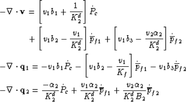
To obtain the b_i, we now combine the above into the macroscopic laws

$$\begin{eqnarray} &&-\nabla \cdot {\bf v} = \left[v_1 b_1 + \frac{1}{K_2^d}\righ... ...}}_{f1} + \frac{v_2 \alpha_2}{K_2^d B_2} \dot{\overline{p}}_{f2} \end{eqnarray}$$ (87) (88) (89)

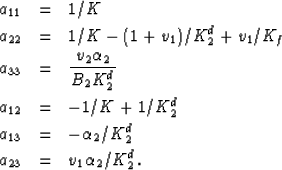
and use the fact that the coefficients of the matrix must be symmetric (a_ij = a_ji). With a₁₁ = 1/K corresponding to the overall drained frame modulus of the composite (to be independently specified), we obtain v₁ b₁ = 1/K - 1/K₂^d, v₁ b₂ = -1/K + (1+v₁)/K₂^d, and $b_3 = - \alpha_2/K_2^d$. The final a_ij coefficients are exactly

$$\begin{eqnarray} a_{11} &=& 1/ K \\ a_{22} &=& 1/K - (1+v_1)/K^d_2 + v_1/K_f \\ ... ...\ a_{13} &=& -\alpha_2/K^d_2 \\ a_{23} &=& {v_1 \alpha_2}/{K^d_2}.\end{eqnarray}$$ (90) (91) (92) (93) (94) (95)

Reasonable models for K and K^d₂ will be discussed shortly.