Dimensionality

A 3-D reflection dataset resides in a five dimensional space. Typically we describe this space in terms of ($t,\bf s,\bf g$) or ($t, \bf h, \bf cmp$) where t is time and $\bf s, \bf g, \bf cmp, \bf h$ are the source, receiver, midpoint, and offset vectors. In Biondi and Vlad (2001) the dimensionality of the dataset was decreased by one by describing offset by a scalar rather than a vector. This is far from an ideal solution, especially in the case of a land dataset and/or data over complicated geology. In both cases the earth being sampled at different azimuths can vary significantly. By stacking we are making an implicit assumption that there isn't any variation (or at least significant variation) due to azimuth. This can affect both our amplitudes and our ability to accurately estimate the model velocity Clapp and Biondi (1995).

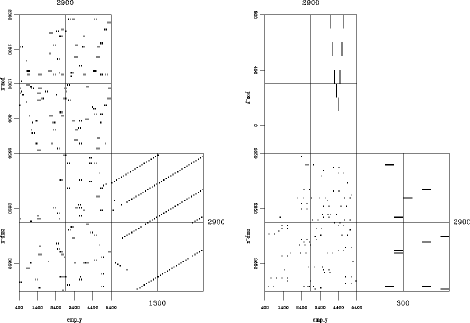
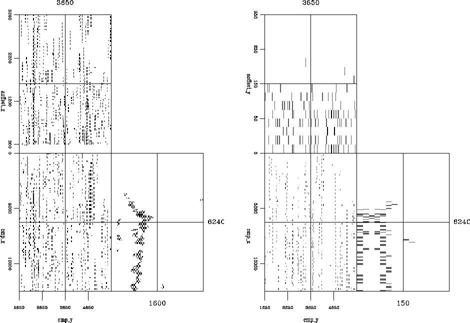
If we use a five dimensional model space we must modify our estimation procedure. The solution is to perform individual estimations at different h_y or azimuths. Solving independent problems is not generally a workable solution. First we aren't imposing any smoothness over h_y or azimuth, something that we know should physically exist. Our estimation procedure is likely to produce an answer far from smooth over the added axes. Figure  and Figure  show fold maps for a portion of a 3-D land and marine datasets. The left panel shows the cmp_x,cmp_y,h_x cube, the latter the cmp_x,cmp_y,h_y cube at the same midpoint location. Note how in both cases the coverage varies significantly as a function of h_y. Take the marine case for example. Standard acquisitions techniques would lead to cmp_y (cross-line direction) locations to be banded along different h_y locations (caused by the multiple towed cables) and few large h_x at small h_y (due to cable feathering).

 

fold.land
Figure 5 The fold from a portion of a 3-D land dataset. The left panel is a subset at a constant h_y. Three panels from the subset are shown. The right panel is a subset at a constant h_x. Both panels show the same cmp_x ,cmp_y location.

 

fold.elf
Figure 6 The fold from a portion of a 3-D marine dataset. The left panel is a subset at a constant h_y. Three panels from the subset are shown. The right panel is a subset at a constant h_x. Both panels show the same cmp_x ,cmp_y locations.