Irregular Traces

Seismic data are recorded as a series of traces that are regularly-sampled in time, but are often spatially distributed in an irregular manner. Since the estimation of a PEF requires a regularly-sampled input, the data are placed on a regular grid. If this grid is too fine to allow a PEF to be estimated, a multi-scale method can be used to introduce more fitting equations Curry and Brown (2001); Curry (2002).

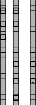
Instead of relying on methods to transform the data onto a regular grid, we can examine if it is possible to manipulate the filter so that it can fit the irregular data. In the case of interlaced data, the filter can be spaced to fit the data. If the data are from a 2D grouping of irregular traces, we can take a small 2-column PEF and dynamically stretch it so that as the filter is convolved with the data, the PEF will always fall on known data.

When looking at 2-column PEF estimation, we can take equation (2) and include a lag matrix $\bf{S}$, which matches the appropriate data point to filter coefficient. For a simple $2 \times 5$ PEF, $\bf{S}$ will look like:  

$$\bold S_{orig} = \left[ \begin{array} {cccccccc} 1 & \cdot... ...cdot & \cdot & \cdot & \cdot & \cdot & 1 \end{array} \right] .$$ (4)

The gap in the diagonal matrix is the length of the n₁ axis (time) minus the filter length in the n₁ dimension. When stretching the data for interlaced traces, the matrix changes, so that  

$$\bold S_{inter} = \left[ \begin{array} {cccccccc} 1 & \cdo... ...cdot & \cdot & \cdot & \cdot & \cdot & 1 \end{array} \right] .$$ (5)

In this case, every second data point is selected by this matrix, and the gap now corresponds to 2 times the length of the n₁ axis, since a row is skipped. Now for a dynamically stretched PEF, the matrix will look somewhat different, as the PEF is not stretched by an integer amount, so if a filter coefficient falls between two data points (as shown in Figure ) a linear combination of the two data points will be multiplied with the PEF coefficient. For a single trace pair, $\bf{S}$ will now be  

$$\bold S_{irreg} = \left[ \begin{array} {cccccccc} 1 & \cdo... ... \cdot & \cdot & \cdot & \cdot & \cdot & 1 \end{array} \right]$$ (6)

 

stretch Figure 2 PEFs on irregular traces. For the first trace pair, the PEF is spaced by 1.5 bins, and for the second the PEF is spaced by 2.25 bins. Where a PEF coefficient falls between data points, a linear combination of the two are used.

if the traces were considered to be 1.5 bins apart. For each trace pair, a separate set of equations where $\bf{Y_{i}}$ corresponds to convolution with the trace pair, $\bf{S_{i}}$ is a filter lag matrix that is a function of the distance between the two traces, $\bf{y_{i}}$ is a copy of the second trace of the pair, and $\bf{K}$ and $\bf{f}$ remain unchanged. For a three-trace set, the fitting goal would be  

$$\bold 0 \quad \approx \quad \bold r = \left[ \begin{array} ... ...} \bf y_1 \\ \bf y_2 \\ \bf y_3 \end{array} \right] .$$ (7)

In methods where the data are transformed to a regular grid Curry and Brown (2001), many parameters (such as scales) need to be chosen. With this method of manipulating the filter to fit the data, the only parameter that needs to be set is the aspect ratio of the PEF, meaning what distance would correspond to a single bin in time.

There are several assumptions being made when estimating a PEF in this manner, most of which are shared with Crawley's 1998 approach. First of all, this method assumes that the filter is scale-invariant, meaning that the stretched filter would behave the same as if it were not stretched, which is valid when dealing with plane waves Claerbout (1999). Next, there is an assumption of stationarity. The filter can be made to be non-stationary, but the stretching of the filter assumes that the area that the stretched filter covers is stationary. Finally, since using a linear combination of two data points as a proxy for a data point located between those two is tantamount to linear interpolation, there is an assumption that the data are not aliased in the well-sampled (time) axis.

There are also several limitations to this approach. First of all, in order to dynamically stretch a PEF to fit data along one dimension, all other dimensions must be regularly-sampled and contain no aliasing. This limits the estimation to 2D with seismic data, since the only dimension with the required regularity is the time axis. This problem can be addressed by simultaneously estimating numerous 2D PEFs for other dimensions. Another issue that arises is multiple dips. A non-stationary filter can deal with different dips in different areas, but is not effective if those dips are co-located. A pair of PEFs could be simultaneously estimated, which might work in estimating both dips.