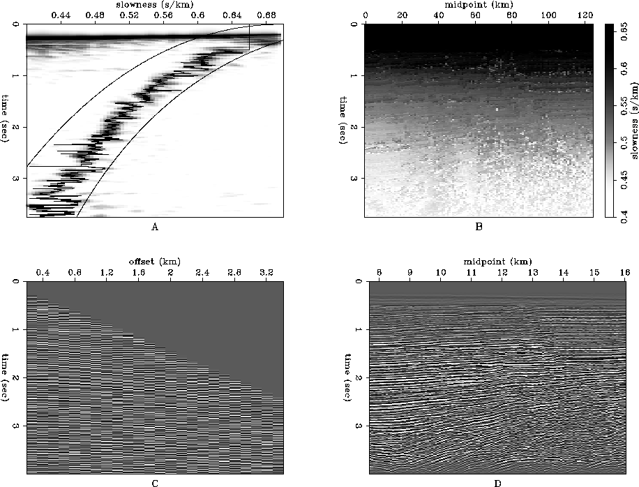
![[*]](http://sepwww.stanford.edu/latex2html/cross_ref_motif.gif) shows the auto-picked RMS velocity and a stack
of the CMP's.
shows the auto-picked RMS velocity and a stack
of the CMP's.
First, we performed velocity analysis on each CMP, and then use an auto-picker
to pick the maximum stacking power that corresponds to the best RMS velocity at each CMP
location. The value of the stacking power at the auto-picked RMS velocity was used as a quality measure of the data, and used as the data residual weight (W) in equations (2), (5), and (8). Clapp (2003) shows an alternative way to calculate the data residual weights based on a multiple realization of the RMS velocity. His approach looks promising since the the RMS velocity average is used as the data and the RMS velocity variance is used as the data residual weight.
Figure ![[*]](http://sepwww.stanford.edu/latex2html/cross_ref_motif.gif) shows the auto-picked RMS velocity and a stack
of the CMP's.
shows the auto-picked RMS velocity and a stack
of the CMP's.
 |
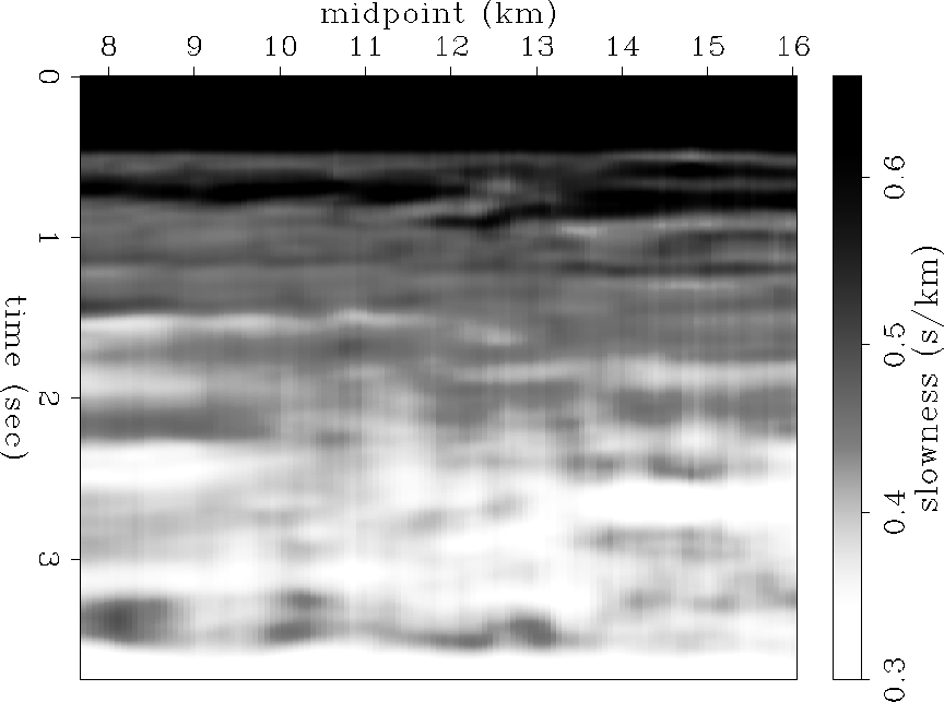
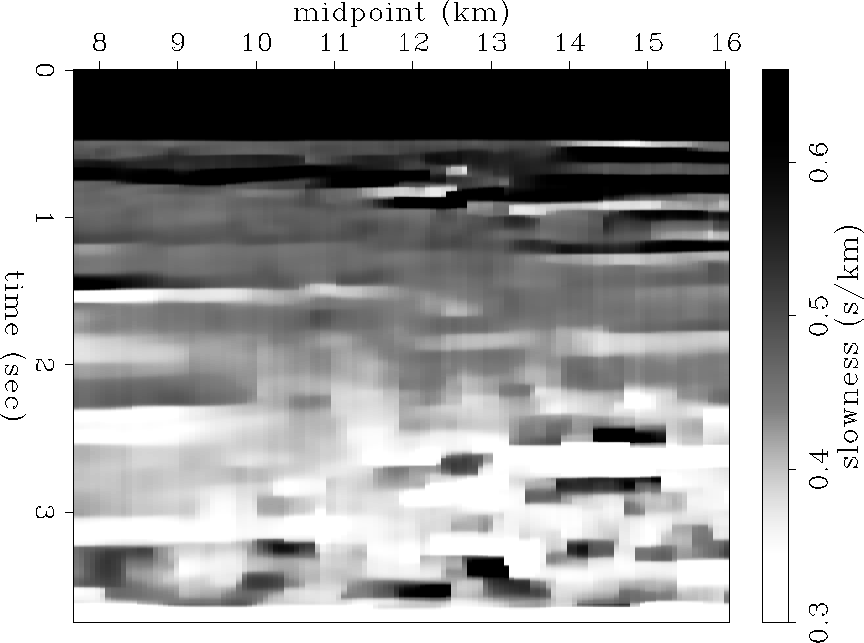
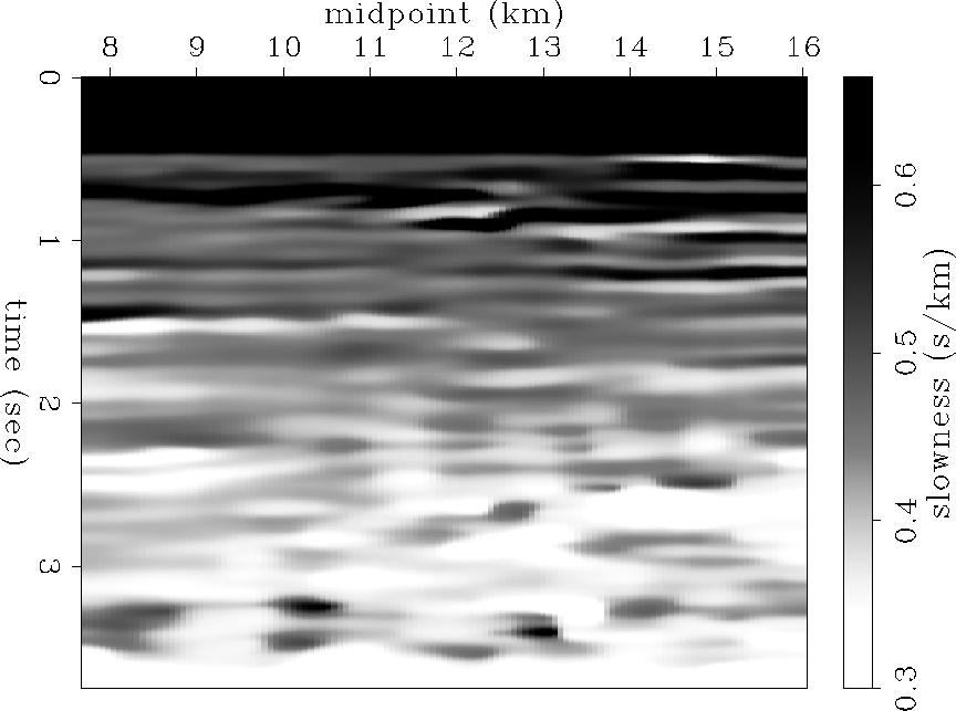
Figures ![[*]](http://sepwww.stanford.edu/latex2html/cross_ref_motif.gif) ,
, ![[*]](http://sepwww.stanford.edu/latex2html/cross_ref_motif.gif) , and
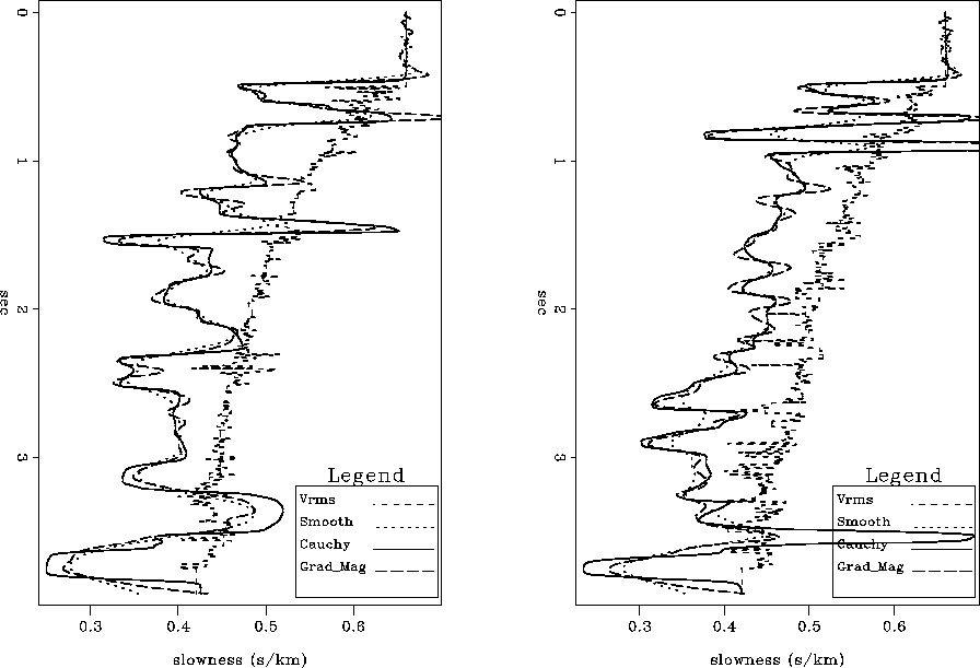
, and ![[*]](http://sepwww.stanford.edu/latex2html/cross_ref_motif.gif) show the interval velocities resulting from solving the inverse problems stated in equations (2), (5), and (8) respectively. We also show in figure
show the interval velocities resulting from solving the inverse problems stated in equations (2), (5), and (8) respectively. We also show in figure ![[*]](http://sepwww.stanford.edu/latex2html/cross_ref_motif.gif) a graph comparing the three methods and the RMS velocity used as input data at two CMP locations.
a graph comparing the three methods and the RMS velocity used as input data at two CMP locations.
 |
![[*]](http://sepwww.stanford.edu/latex2html/movie.gif)
 |
![[*]](http://sepwww.stanford.edu/latex2html/movie.gif)
 |
![[*]](http://sepwww.stanford.edu/latex2html/movie.gif)
 |
The resulting interval velocity models show what the regularization was designed to do. In figure ![[*]](http://sepwww.stanford.edu/latex2html/cross_ref_motif.gif) the resulting interval velocity is smooth in time and space. Figure
the resulting interval velocity is smooth in time and space. Figure ![[*]](http://sepwww.stanford.edu/latex2html/cross_ref_motif.gif) shows sharp edged rectangular shapes all over the image, looking reasonable in the faults but in general geological unappealing. Figure
shows sharp edged rectangular shapes all over the image, looking reasonable in the faults but in general geological unappealing. Figure ![[*]](http://sepwww.stanford.edu/latex2html/cross_ref_motif.gif) shows sharp objects with more geological appeal.
shows sharp objects with more geological appeal.
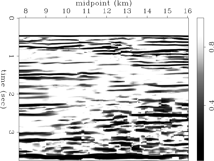
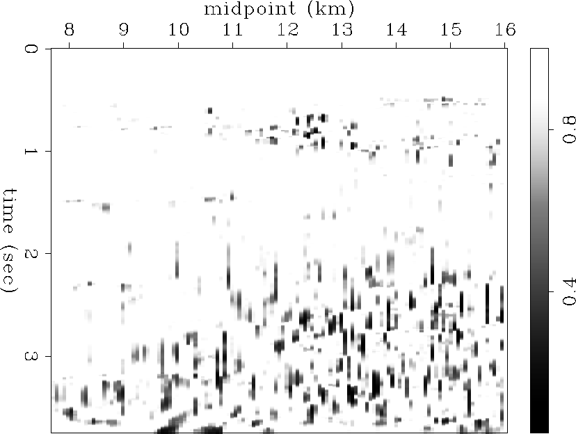
The preferential shapes can also be seen in the diagonal weight operator. Figures ![[*]](http://sepwww.stanford.edu/latex2html/cross_ref_motif.gif) and
and ![[*]](http://sepwww.stanford.edu/latex2html/cross_ref_motif.gif) show
show ![]() and
and ![]() , the last nonlinear iteration diagonal weight operator in equation (7). Notice the two preferential directions in what the edges are preserved. Figure
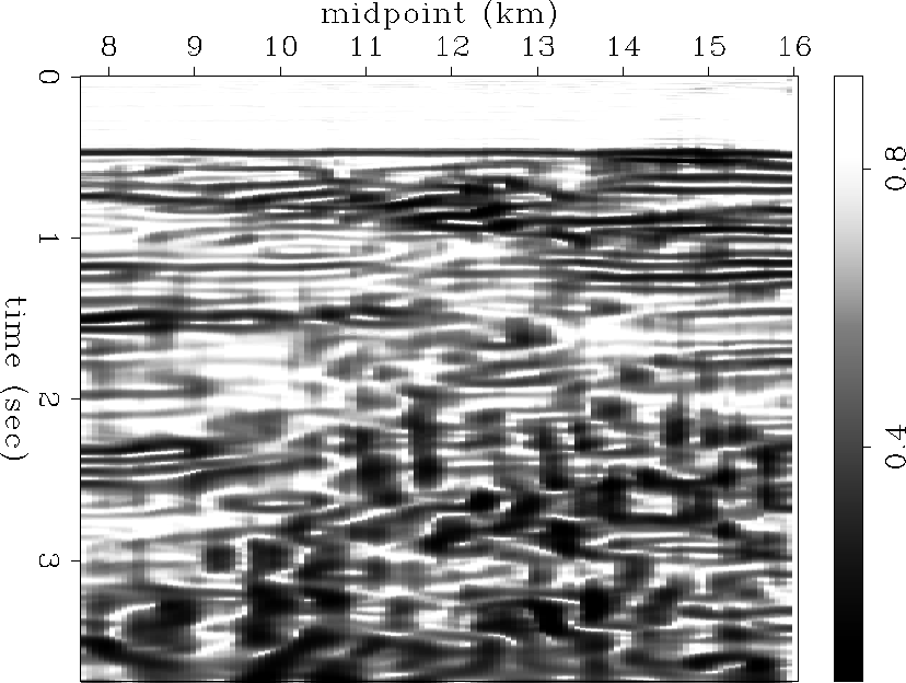
, the last nonlinear iteration diagonal weight operator in equation (7). Notice the two preferential directions in what the edges are preserved. Figure ![[*]](http://sepwww.stanford.edu/latex2html/cross_ref_motif.gif) shows
shows ![]() , the last nonlinear iteration diagonal weight operator in equation (9). Notice the isotropic behavior of the diagonal weight calculated using the gradient magnitude operator.
, the last nonlinear iteration diagonal weight operator in equation (9). Notice the isotropic behavior of the diagonal weight calculated using the gradient magnitude operator.
 |
 |
 |