Background

Sparse data interpolation is a very important problem in geophysics, due to the high cost associated with data collection. Irregular sampling introduces another level of complexity to the problem. Data interpolation can be implemented using a two stage linear method, the second of which is the minimization of the model when convolved with a filter. The first step is determining an appropriate filter, such as a prediction-error filter (PEF) Claerbout (1999).

A PEF can often be estimated by minimizing the output of convolution of an unknown filter with known data. The one dimensional case,

 

$$\bold 0 \quad \approx \quad \bold r = \left[ \begin{array} ... ..._2 \\ y_3 \\ y_4 \\ y_5 \\ y_6 \end{array} \right]$$ (1)

can easily be extended to multiple dimensions with the helical coordinate Claerbout (1998). Here a represents filter coefficients, y represents data, and $\bf r$ is the residual, which we minimize. When there are unknown data, the equations containing missing data are not used. Very sparse data complicates the issue, since there are no fitting equations which determine a PEF. Looking at the above equation, if y₂, y₃ and y₄ were missing, a PEF could not be determined.

A method to overcome the need for contiguous data is to stretch the filter Crawley (1998) so that the filter coefficients would fall upon data points. The stretching can be done at multiple scales, due the the scale-invariance of the PEF Claerbout (1999). This method works well as long as the data are regularly sampled, and the stretching is isotropic. If the data are irregularly sampled, the method fails, since the filter coefficients no longer fall upon data points, and again we are left without fitting equations.

$$\begin{array} {ccccccccc} &\cdot &a &\cdot &b &\cdot &c &\cd... ...dot &\cdot &\cdot &1 &\cdot &\cdot &\cdot &\cdot \\ \end{array}$$

 

peffail
Figure 1 Figure of three cases for a regression equation. The diagonal lines represent gridded data, the white squares are empty bins, and the bold lines represent the PEF. Left: Original PEF on interlaced data, where an equation is not possible. Center: scale-expanded PEF on interlaced data, with a possible equation. Right: scale-expanded PEF on irregularly spaced data, no equation is possible.

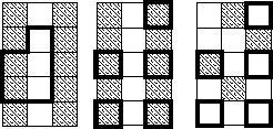
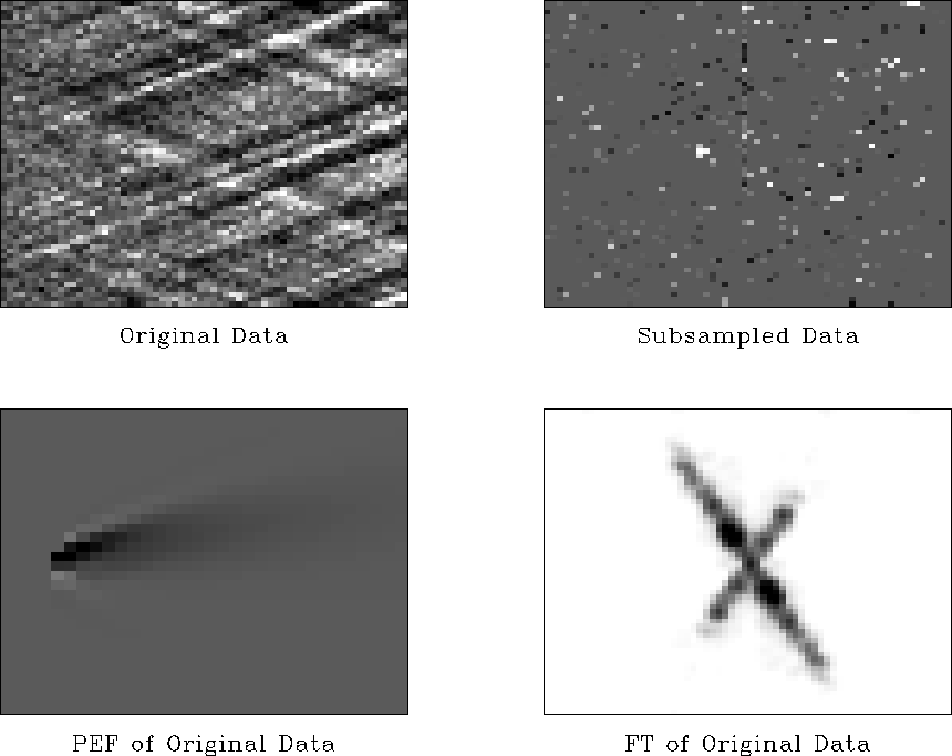
A test case has been developed Brown et al. (2000), which consists of a single plane wave oriented at 22.5^o, irregularly sampled. We extend this test case, and add complexity to it by adding another plane wave with a different frequency and orientation. In addition we add a substantial amount of Gaussian noise. Crawley's 1998 method of scaling the filter does not work for this case, as the irregular sampling leads to a lack of fitting equations. The sampling is much like the middle case in Figure 1 where the filter does not lie on known data, regardless of how much it is stretched.

 

data
Figure 2 Clockwise from top left: Fully sampled test data; Sparsely sampled test data; Envelope of Fourier Transform of fully sampled test data, Inverse impulse response of PEF from all data.