One-dimensional synthetic examples

The simple test examples in this section are borrowed from Claerbout (1999).

 

data Figure 1 The input data (right) are irregularly spaced samples of a sinusoid (left).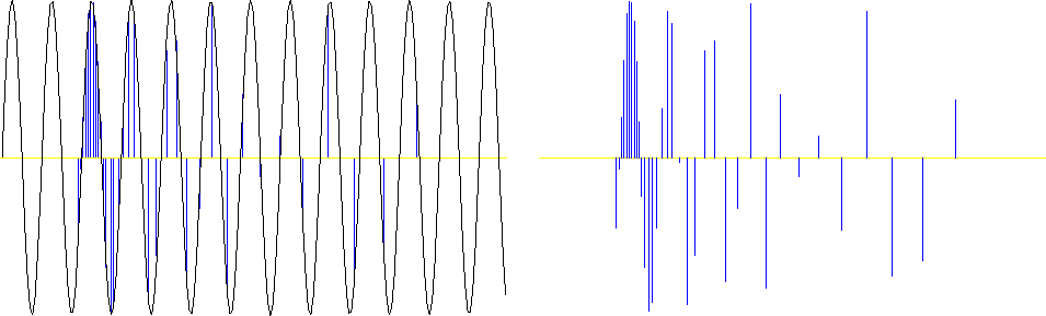

In the first example, the input data were randomly subsampled (with decreasing density) from a sinusoid (Figure ). The forward operator $\bold{L}$ in this case is linear interpolation. In other words, we seek a regularly sampled model on 200 grid points that could predict the data with a forward linear interpolation. Sparse irregular distribution of the input data makes the regularization enforcement a necessity. Following Claerbout (1999), I applied convolution with the simple (1,-1) difference filter as the operator $\bold{D}$ that forces model continuity (the first-order spline). An appropriate preconditioner $\bold{P}$ in this case is recursive causal integration. Figures and show the results of inverse interpolation after exhaustive 300 iterations of the conjugate-direction method. The results from the model-space and data-space regularization look similar except for the boundary conditions outside the data range. As a result of using the causal integration for preconditioning, the rightmost part of the model in the data-space case stays at a constant level instead of decreasing to zero. If we specifically wanted a zero-value boundary condition, we could easily implement it by adding a zero-value data point at the boundary.

 

im1 Figure 2 Estimation of a continuous function by the model-space regularization. The difference operator $\bold{D}$ is the derivative operator (convolution with (1,-1)).

 

fm1 Figure 3 Estimation of a continuous function by the data-space regularization. The preconditioning operator 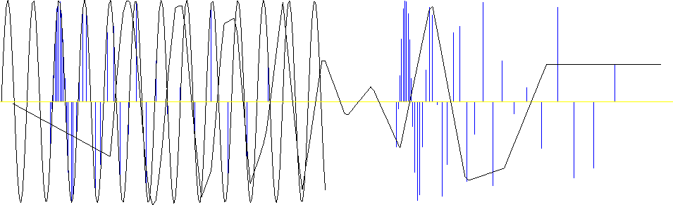$\bold{P}$ is causal integration.

As expected from the general theory, the model preconditioning provides a much faster rate of convergence. I measured the rate of convergence using the model residual, which is a distance from the current model to the final solution. Figure shows that the preconditioning (data regularization) method converged to the final solution in about 6 times fewer iterations than the model regularization. Since the cost of each iteration for each method is roughly equal, the computational economy is evident. Figure shows the final solution, and the estimates from model- and data-space regularization after only 5 iterations of conjugate directions. The data-space estimate looks much closer to the final solution than its competitor.

 

early1
Figure 4 The top figure is the exact solution found in 250 iterations. The middle is with data-space regularization after 5 iterations. The bottom is with model-space regularization after 5 iterations.

 

schwab1 Figure 5 Convergence of the iterative optimization, measured in terms of the model residual. The ``d'' points stand for data-space regularization; the ``m'' points for model-space regularization.

Changing the preconditioning operator changes the regularization result. Figure shows the result of data-space regularization after a triangle smoother is applied as the model preconditioner. Triangle smoother is a filter with the Z-transform $\frac{\left(1-Z^N\right)\left(1-Z^{-N}\right)}{(1-Z)\left(1-Z^{-1}\right)}$Claerbout (1992). I chose the filter length N=6.

 

fm6 Figure 6 Estimation of a smooth function by the data-space regularization. The preconditioning operator $\bold{P}$ is a triangle smoother.

If, instead of looking for a smooth interpolation, we want to limit the number of frequency components, then the best choice for the model-space regularization operator $\bold{D}$ is a prediction-error filter (PEF). To obtain a mono-frequency output, we can use a three-point PEF, which has the Z-transform representation D (Z) = 1 + a₁ Z + a₂ Z². In this case, the corresponding preconditioner P could be the three-point recursive filter P (Z) = 1 / (1 + a₁ Z + a₂ Z²). To test this idea, I estimated the PEF D (Z) from the output of inverse linear interpolation (Figure ), and ran the data-space regularized estimation again, substituting the recursive filter P (Z) = 1/ D(Z) in place of the causal integration. I repeated this two-step procedure three times to get a better estimate for the PEF. The result, shown in Figure , exhibits the desired mono-frequency output.

 

pm1 Figure 7 Estimation of a mono-frequency function by the data-space regularization. The preconditioning operator 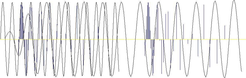$\bold{P}$ is a recursive filter (the inverse of PEF).