


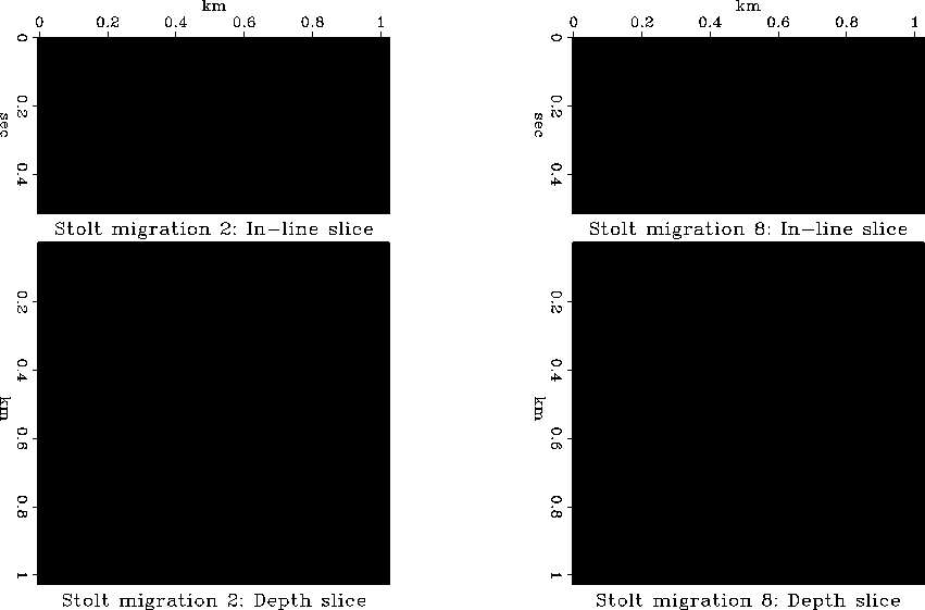
For completeness, I conclude this section with two simple examples of forward interpolation in seismic data processing. Figure 27 shows a 3-D impulse response of Stolt migration (), computed by using 2-point linear interpolation and 8-point B-spline interpolation. As noted by () and (), inaccurate interpolation may lead to spurious artifact events in Stolt-migrated images. Indeed, we see several artifacts in the image with linear interpolation (the left plots in Figure 27). The artifacts are removed if we use a more accurate interpolation method (the right plots in Figure 27).
 |


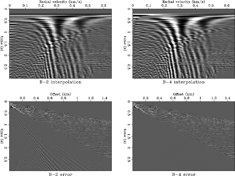
Another simple example is the radial trace transform (). Figure 28 shows a land shot gather contaminated by nearly radial ground-roll. As discussed by (), (, ), and (, ), one can effectively eliminate ground-roll noise by applying a radial trace transform followed by high-pass filtering and the inverse radial transform. Figure 29 shows the result of the forward radial transform of the shot gather in Figure 28 in the radial band of the ground-roll noise and the transform error after we go back to the original domain. Comparing the results of using linear and third-order B-spline interpolation, we see once again that the transform artifacts are removed with a more accurate interpolation scheme.
|
radialdat
Figure 28 Ground-roll-contaminated shot gather used in a radial transform test | 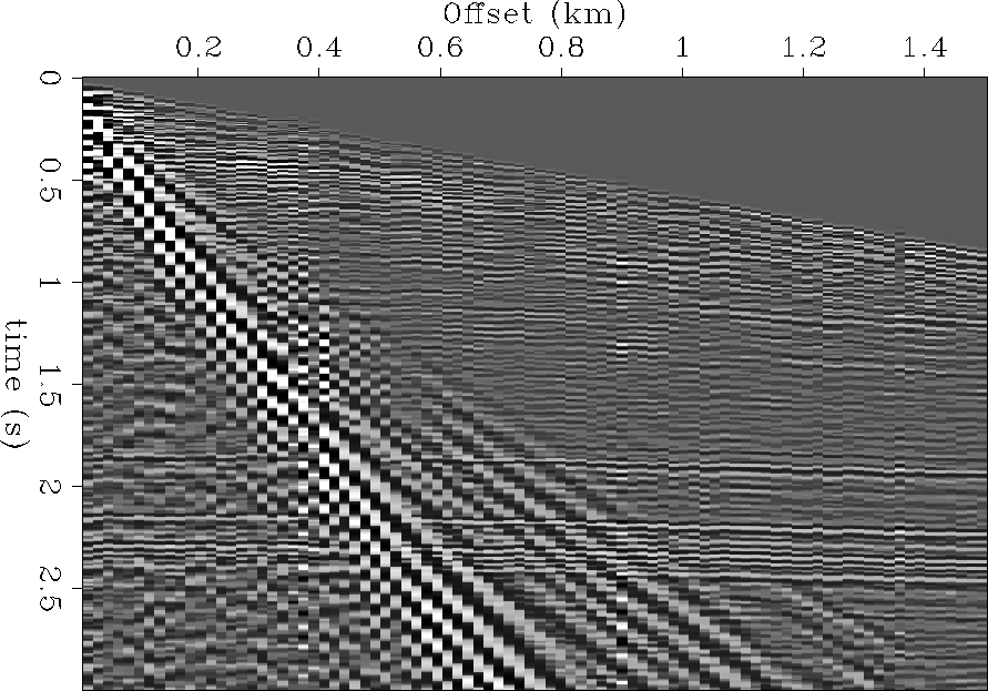 |
 |