![[*]](http://sepwww.stanford.edu/latex2html/cross_ref_motif.gif) . I first calculated the dip along
the nine non-salt reflectors
and then interpolated to the entire model space.
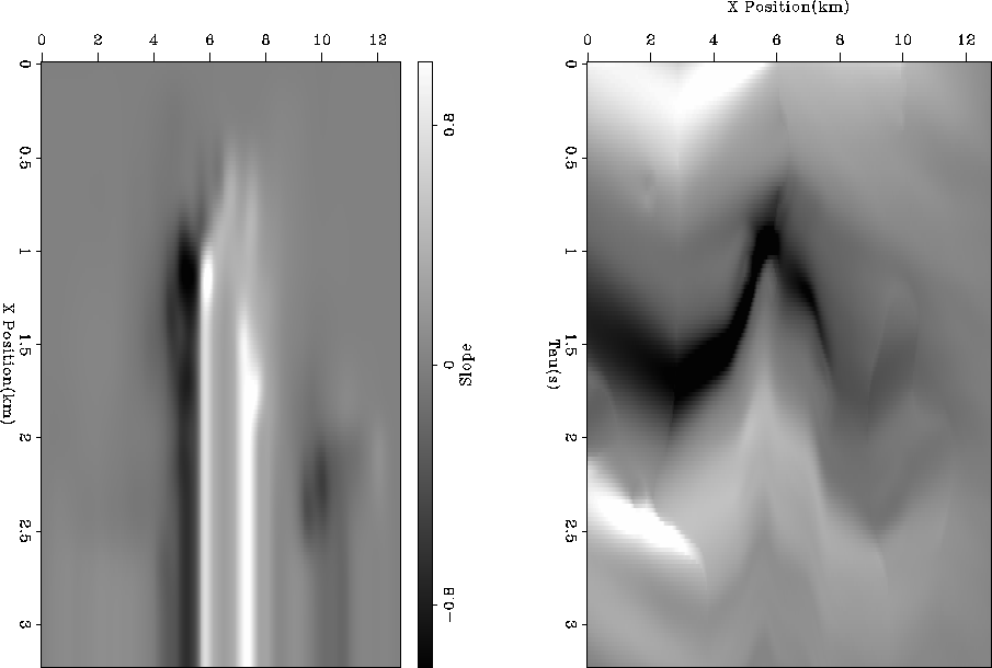
Figure 7 shows the interpolated dip field and
the result of applying
. I first calculated the dip along
the nine non-salt reflectors
and then interpolated to the entire model space.
Figure 7 shows the interpolated dip field and
the result of applying
For constructing the steering filters I used the same methodology as
described in Chapter ![[*]](http://sepwww.stanford.edu/latex2html/cross_ref_motif.gif) . I first calculated the dip along
the nine non-salt reflectors
and then interpolated to the entire model space.
Figure 7 shows the interpolated dip field and
the result of applying
. I first calculated the dip along
the nine non-salt reflectors
and then interpolated to the entire model space.
Figure 7 shows the interpolated dip field and
the result of applying ![]() to random noise. As you
can see the preconditioning operator tends to create low frequency
changes fairly flat in the left portion of the model and more ``U'' shaped
changes to the right of the salt.
to random noise. As you
can see the preconditioning operator tends to create low frequency
changes fairly flat in the left portion of the model and more ``U'' shaped
changes to the right of the salt.
 |
![[*]](http://sepwww.stanford.edu/latex2html/movie.gif)
The salt and salt boundary added additional complications.
The sediment velocity abutting the salt dome is
significantly different from the salt velocity. Using fitting
goals (![[*]](http://sepwww.stanford.edu/latex2html/cross_ref_motif.gif) ) would create a smooth transition
from the sediment layers to the salt velocity instead of the sharp
contrast that often occurs when salt intrudes into
sediments of significantly lower velocity. As a result it was necessary to
make a slight modification to the tomography fitting goals.
) would create a smooth transition
from the sediment layers to the salt velocity instead of the sharp
contrast that often occurs when salt intrudes into
sediments of significantly lower velocity. As a result it was necessary to
make a slight modification to the tomography fitting goals.
I introduced a new diagonal operator ![]() , which is large
where we want model smoothness and becomes smaller as we approach
the salt boundary.
Adding this operator to the model styling goal and then applying
the same preconditioning trick we end up with
, which is large
where we want model smoothness and becomes smaller as we approach
the salt boundary.
Adding this operator to the model styling goal and then applying
the same preconditioning trick we end up with
| |
||
| (1) |
The salt itself was an additional complication. Normally salt velocity is fairly constant. Reflector continuity disappears (and therefore can not be used reliably by the tomography operator) as we get close to the salt boundary and in lower portions of the model. Very few of the raypaths used in tomography pass through the salt structure. As a result the model fitting goal would be dominated by the model styling goal and instead of a constant velocity function we would get unrealistic smooth variation in the salt velocity. To counter this problem, I followed the common practice of not allowing the salt velocity to vary.