Introduction and summary

The tomography method described in the preceding chapter is suited for a particular class of problem. Generating raypaths and picking reflectors requires the dataset to be relatively clean with strong, fairly continuous reflectors. Formulating the tomography in tau is universally advantageous, but shows the most significant improvement over conventional techniques when velocity is not monotonically increasing. Finally, this method assumes that velocity generally follows structural dip, making a steering filter an effective regularization operator.

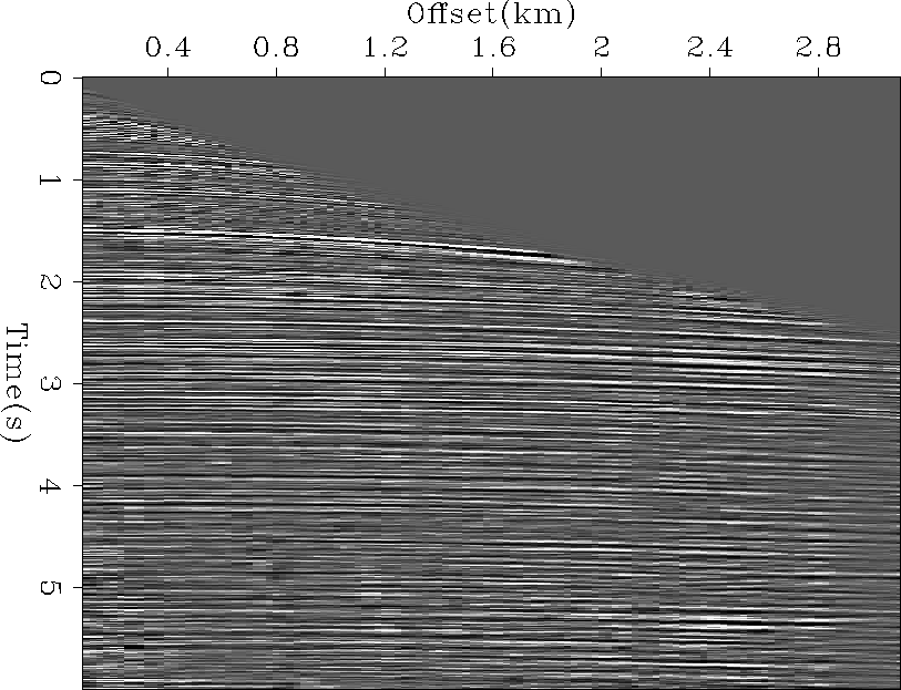
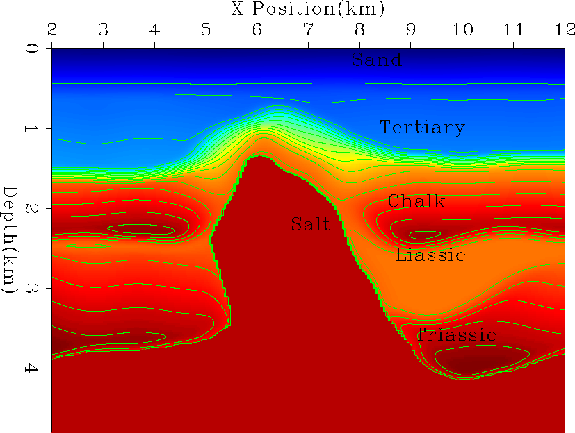
The North Sea dataset provided to SEP by TotalFinaElf. meets all of these criteria. The data is very clean (Figure 1) with strong reflectors that are generally continuous. The data contains a chalk layer which causes a velocity inversion below it. The initial velocity model (Figure 2) was created by IFP using the S.M.A.R.T method (, ). The velocity structure shows typical North Sea behavior with velocity following structural layers.

 

elf-shot Figure 1 A preprocessed shot gather from the L7D dataset.

 

vel0 Figure 2 The initial velocity model for the 2-D line. Overlaid are the general geologic units in the area. Note how the velocity follows structural dip and that velocity decrease below the chalk layer in the Liassic.

The dataset is 3-D marine acquired using four cables with geophones every 25 meters. In this chapter I will be dealing with a 2-D subset of the 3-D dataset. The line was chosen to coincide with a 2-D synthetic dataset (, ). The subset was created by forming partial stacking and then applying Azimuth Moveout (AMO) () to the CMP gathers.

I will begin this chapter by showing the migration and moveout errors with the initial velocity. Next, I will show how I built the steering filter operator and some of the issues involved in dealing with the complex salt structure. I will then move onto applying the tomography technique to the dataset.