


If you can interpolate noisy data, then it is natural to think about interpolating land data. Land data can be difficult and time-consuming to acquire, depending on the survey area, so naturally it is attractive to acquire less of it in the field. Unfortunately, land data is also much harder to interpolate, for a number of reasons. First, land geometries tend not to be well-behaved in the way that marine geometries are. Marine cables are all the same length, and are dragged through the water while recording, so that there is a restoring force working against sharp bends in the receiver lines, smoothing them out. Land geophones are static; they do not have anything smoothing out the kinks in the receiver lines. Sharp bends are common, as are receiver lines of different lengths, and large static shifts. Taken together, these things mean that land data does not have the same kind of lateral coherence and predictable acquisition that makes marine data ideal for interpolation. Nonetheless, because of the expense and effort of acquiring land data, it is worthwhile to try interpolating it.
Arabian data examples
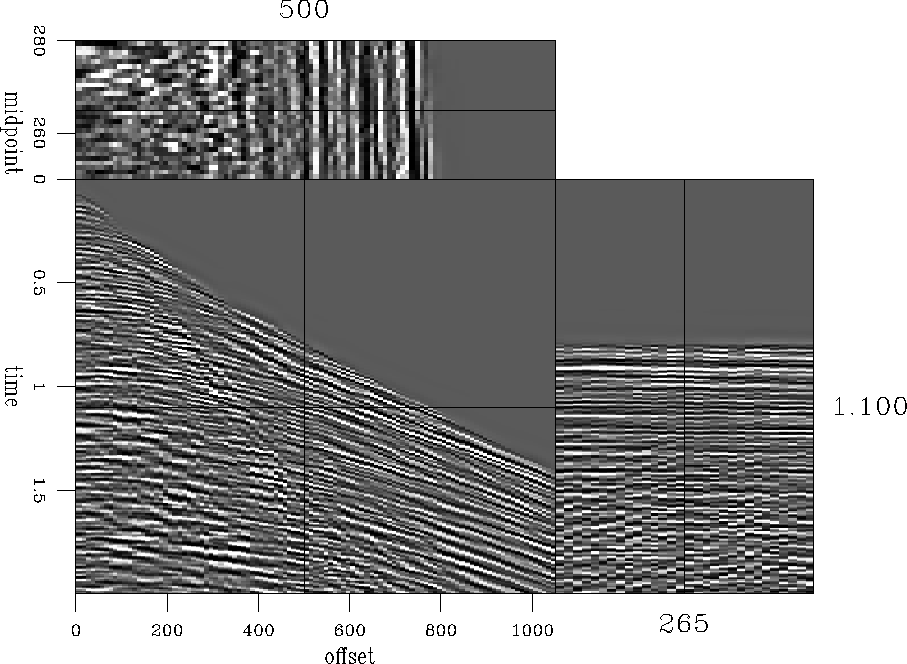
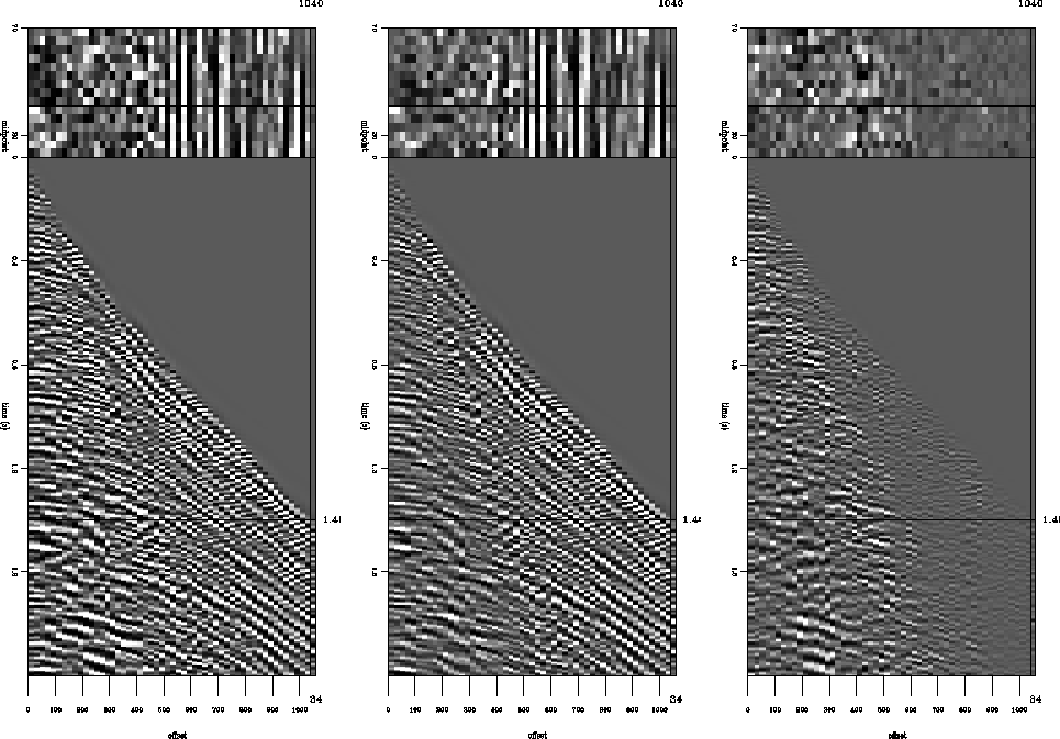
The first land data examples are from a data set from Saudi Arabia, which has a mostly regular geometry, and is very clean for land data. The first is made up of all the positive offsets from a set of CMP gathers, shown in Figure sgyWin2.in. This data is divisible by inspection into two wedge-shaped regions. The nearer offset wedge is the noisier of the two; it contains the surface waves. The farther offset wedge is outside the cone of surface waves, and appears very clean. In the coherent wedge towards farther offsets, events are predictable both in offset and in midpoint. In the near offset wedge, events are predictable only over much shorter distances in offset, and are unpredictable in midpoint. Figure sgyWin2.out shows portions of the original and interpolated data cubes. The data in Figure sgyWin2.out is subsampled so that only missing traces are shown. The left panel shows some of the traces which were removed from the original data to make the input cube. The center panel shows those same traces taken from the interpolation result, and the right panel shows the difference. There are large differences, though they are mostly incoherent, and mostly restricted to the noisy inner offsets. Most of the somewhat coherent noise events visible in the original data are interpolated, though not fully. For instance, there are a number of nearly horizontal events near the bottom of the input traces, in the inner half of the offsets, each about five traces wide in offset, and one trace wide in midpoint. These events are visible in the output, but their amplitudes are lower than in the input. Over the whole input, about 72% of the variance is predicted.
 |

 |
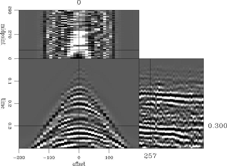
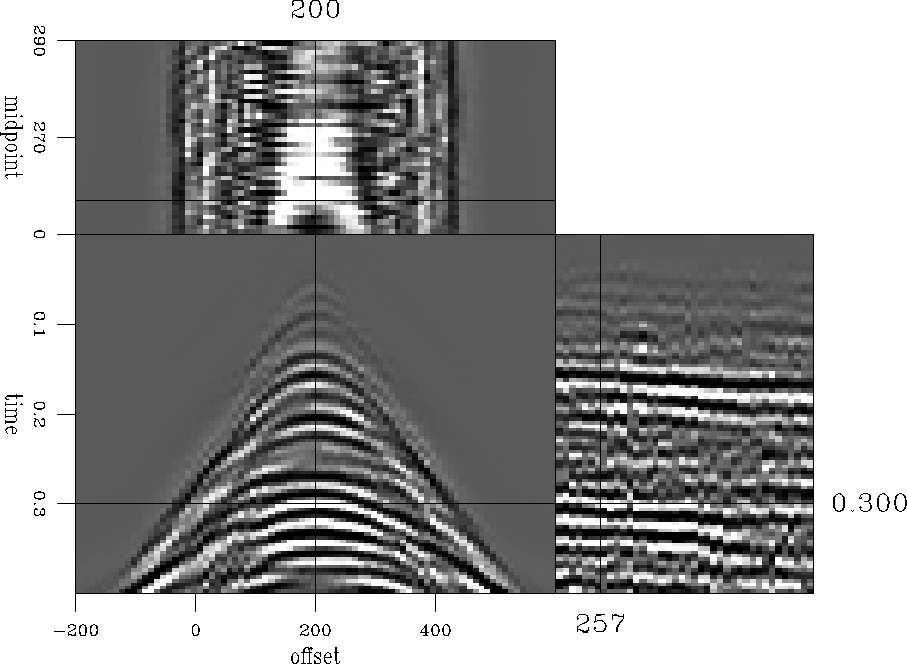
The next figures zoom in on the near offset, short time portion of the data, where there is the strongest curvature. Figures sgyWin1.in and sgyWin1.out show input and output cubes where the data are just the near offsets and short times of some CMP gathers. In this case offsets are interpolated instead of shots; the data are CMP gathers, and the shot and receiver spacings are equal, so the fold is equal to half the number of receivers. Here we just double the fold. We do not begin by subsampling the known data, so there are not any obvious input/output comparisons. It is just presented as an exercise in interpolating strongly curved, somewhat aliased events. At any rate, the result is convincing, if subjective.
 |
 |
Arizona data example
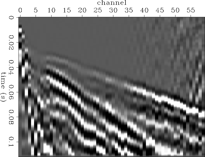
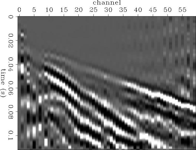
The last example uses an environmental data set acquired near a copper mine in Arizona. The data was acquired on rough terrain. There are large statics throughout the data, and the geometry is much less predictable than in a marine case, or in the Saudi data.
In this data set, receivers were zeroed in a checkerboard pattern and reinterpolated, similar to several earlier experiments on marine data. This survey used a roll switch to increment the active receiver range with each shot, so the geometry is similar to a marine survey in the sense that the offset range is the same on each shot gather. This subsampling can thus simulate half as many receiver locations or half as many shots with the input taken to be receiver gathers rather than shot gathers. Unlike the marine case, the ground surface where this data was recorded is rough, so that the geometry does not have the regularity of earlier examples. The rough surface and the relatively unpredictable geometry give rise to statics and scattered noise in the data, which make it difficult to predict. As a result, the interpolation is not perfect, with 75% of the variance predicted. Nevertheless, it is good, given the input.
Figure minetestin shows a shot gather from the original input data. Figure minetestout shows the same view of the output, after subsampling and interpolating. The most obvious difference is at the very closest offsets. Here events dip so steeply that they are beyond the angular range of the PEFs used to interpolate, so nothing is filled in. A more subtle difference is the static shifts between original traces and their interpolated counterparts. Interpolated traces may have the correct waveform, but not the correct static shift relative to surrounding traces. Figure minetestout is a two-frame movie in the electronic version of this document. Flipping between the two frames you can see that several channels have statics in the original data which are not present in the interpolated trace. The possibility of introducing non-surface-consistent statics in this way is an interesting, unexplored topic.
 |
 |