|
mod1.refl
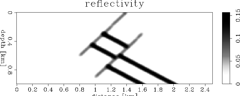
Figure 4 The reflectivity model. |  |
|
mod1.refl
Figure 4 The reflectivity model. |  |
|
mod1.Slow.0
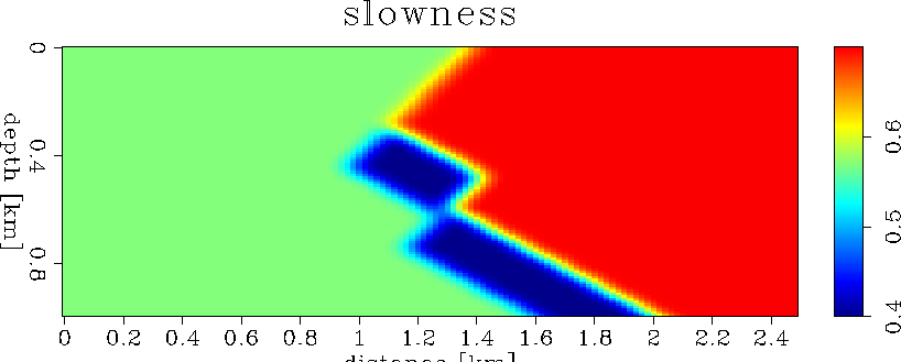
Figure 5 The true slowness model. |  |
We begin by generating a synthetic dataset. Based on our simulated acquisition, defined by a half-offset of 2.0 km, we expect to achieve a reasonably good angular coverage of the region of interest, which is not deep.
The goal of this test is to start the imaging process by assuming that we don't know much about the slowness of the fast layer and to use our technique to fill the missing slowness. We run two separate tests: a simpler test when we assume that we know the geometry and slowness of the upper part of the model, and a more complex test when we do not assume anything about the slowness in the layer and attempt to fill it out entirely. ![[*]](http://sepwww.stanford.edu/latex2html/foot_motif.gif)