Inversion in the reflection angle domain

Since we are using this method to image complex areas, just performing migration is not enough Prucha et al. (1999). We want to formulate the process as an inversion problem Duquet and Marfurt (1999); Nemeth et al. (1999). Unfortunately, the complexity can cause the result of the inversion to diverge. Therefore, to constrain the inversion to a reasonable result, we choose to impose regularization. This can be represented by these fitting goals:

$$\begin{eqnarray} {\bf d \approx Lm} \\ 0 \approx \epsilon {\bf A m}\end{eqnarray}$$ (6) (7)

where ${\bf d}$ is the data space, ${\bf m}$ is the model space, ${\bf L}$ is the wave-equation operator, ${\bf A}$ is the regularization operator, and choosing the parameter $\epsilon$ is a Lagrange multiplier that allows us to determine how strong our regularization (smoothing) will be.

To speed the convergence of the inversion, we can reformulate the inversion problem as a preconditioning problem with a preconditioning operator ${\bf S}$. This operator should be as close to the inverse of the regularization operator as possible so that ${\bf AS \approx I}$. By mapping the multi-dimensional regularization operator ${\bf A}$ to helical space and applying polynomial division, we can obtain the exact inverse so that ${\bf S = A^{-1}}$ Claerbout (1998). We also use the preconditioning transformation ${\bf m = Sp}$ Fomel et al. (1997). Our equations then become:

$$\begin{eqnarray} {\bf d \approx LSp} \\ 0 \approx \epsilon {\bf p}.\end{eqnarray}$$ (8) (9)

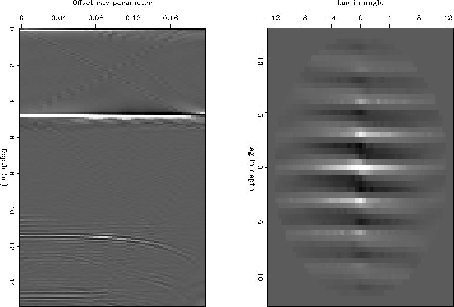
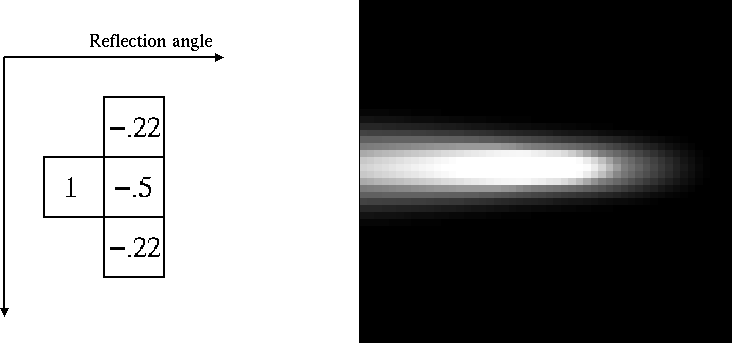
The regularization we choose for RAD inversion is horizontal smoothing along the reflection angle (or p_hx) axis. This is based on both theory and practice. In theory, the regularization operator should be related to the inverse model covariance matrix Tarantola (1986). In practice, because the covariance matrix of a CIG created with the correct velocity model is horizontal in nature (Figure 2) and the reflectivity along reflection angles should vary smoothly Richter (1941), we simply smooth horizontally along the reflection angle axis. An operator that fulfills these requirements is a steering filter Clapp et al. (1997). This steering filter and its impulse response is in Figure 3. The coefficients in the second column of the steering filter are variable and control the vertical width of the impulse response.

 

covar
Figure 2 Left: a typical RAD CIG with some minor artifacts. Right: representation of the covariance matrix calculated for this CIG.

 

filtres
Figure 3 Left: steering filter used for regularization. Right: impulse response of steering filter.

We also must choose an $\epsilon$. A large $\epsilon$ means that the regularization will be strong (we will be smoothing more) and a small $\epsilon$ means the regularization is not strong (we honor the model more). For now, we are trying to choose an $\epsilon$ that is somewhere in the middle, so that our result is slightly smoothed. We want to try to fill the null space in a reasonable way.