Examples

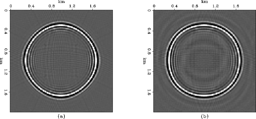
Figure 1 compares depth-slices through impulse responses of FFD migration (with c/v=0.8) for the splitting approximation, (a), and the helical factorization, (b). The azimuthal anisotropy is noticeably reduced with the helical factorization.

 

timeslices
Figure 1 Depth-slices of centered impulse response corresponding to a dip of 45 for c/v=0.8. Panel (a) shows the result of employing an x-y splitting approximation, and panel (b) shows the result of the helical factorization. Note the azimuthally isotropic nature of panel (b).

Figure 2 shows extracts from a three-dimensional FFD depth migration of a zero-offset subset from the SEG/EAGE salt dome dataset. This rugose lateral velocity model initially caused mild stability problems for the FFD migration, and I had to smooth the velocity model to produce the results shown in Figure 2. Biondi (2000) presents an unconditionally stable formulation of the FFD algorithm; however, that formulation does not easily fit with the approximate helical factorization discussed here.