 |
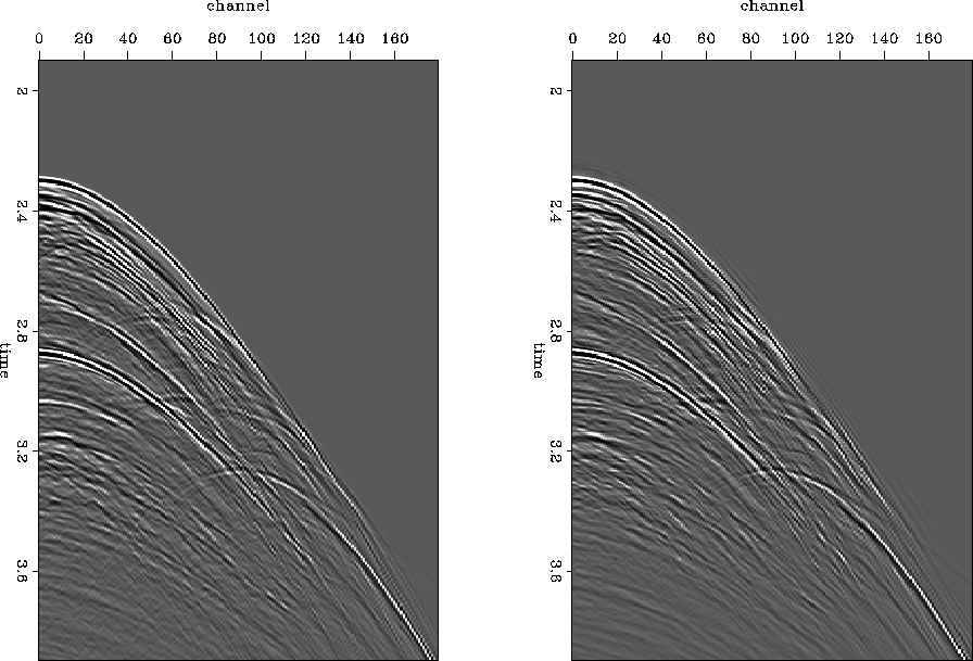
Figure 3 Interpolation test. Left panel is a shot gather that was removed from the input data. Right panel is the interpolated version of that shot gather.
In the previous example, I could throw away lots of data and restore it pretty faithfully, because the data is very predictable. In time slice view, it is almost entirely straight lines. The geology in that example is flat, so it is probably not necessary to think about multiples in three dimensions. The next example is from a marine survey over much more complex geology, where multiple energy moving in three dimensions could be a genuine concern. It is just a 2-D survey; I simulate one inline from a survey with four sources by throwing away three out of four shot gathers. I then attempt to reconstruct the data. Some results are shown in Figures 355Fig2b, 355Fig2, and 355Fig1. In this example, the data are reduced to every fourth shot gather and interpolated back to every second shot gather. If that works, then getting from every second shot to every shot is fairly certain. There is no conceptual reason not to go directly from every fourth shot to every shot in a single step, it just means scaling the axes by four rather than two. There is a practical issue that arises, however, in that filter coefficients are smoothed by a variant of leaky integration, and there tends to be a little too much leakage.
Figures 355Fig2b and 355Fig2 show shot gathers that were removed in the left panels, and the interpolated versions of those shot gathers in the right panels. The result are not bad, but not perfect, either. Surprisingly little energy dipping in towards zero offset is lost; given the particular filter smoothing strategy I use, I expected those events to be lost. However, several events close to zero offset are poorly reconstructed.
Figure 355Fig1 shows a time slice from the correct (recorded) data in the left panel, the input to the interpolation in the middle, and the interpolation on the right. Again the output is not bad, but not flawless either. The spatial frequencies are too low near zero offset, for instance.
 |
 |
 |