Examples

In this section, I present two 2-D post-stack synthetic examples, shown in Figures 2 and 3, to prove the applicability of the equations derived in the preceding sections.

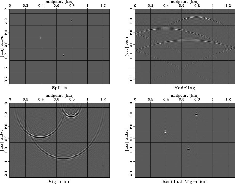
In the first example, the input is a set of three spikes. Initially, I do forward modeling with a velocity of v_m=3.0 km/s. Next, I do Stolt migration with a velocity of v₀=3.6 km/s, and residual Stolt migration with a ratio v₀/v_m=1.2 (Figure 2). I then take the same input and perform Stolt migration with a velocity of v₀=2.4 km/s, followed by residual Stolt migration with a ratio v₀/v_m=0.8 (Figure 3). In both cases, the data are correctly collapsed at the location of the original spikes. Residual migration can be done without knowing the absolute values of the velocity.

 

posp
Figure 2 Top left: input data. Top right: Stolt forward modeling with the correct velocity v_m=3.0 km/s. Bottom left: Stolt migration with an incorrect velocity of v₀=3.6 km/s. Bottom right: Stolt residual migration with the ratio v₀/v_m=1.2.

 

posm
Figure 3 Top left: input data. Top right: Stolt forward modeling with the correct velocity v_m=3.0 km/s. Bottom left: Stolt migration with an incorrect velocity of v₀=2.4 km/s. Bottom right: Stolt residual migration with the ratio v₀/v_m=0.8.

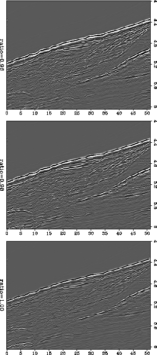
In the next example, shown in Figure 4, I apply the same methodology to a real dataset Ecker (1998). All three panels are the result of residual migration as described in the preceding theory sections. The corresponding ratios are 0.96 for the top panel, 0.98 for middle panel, and 1.00 for the bottom panel. Residual migration with ratio=1.0 is equivalent to no residual migration at all. It is apparent that different images are focused better in one region or another, although the image corresponding to the ratio 0.98 seems to have the highest overall energy. We can use such an observation to obtain an image that has the best focusing in all the regions. This can be achieved by doing residual migration for a range of velocity ratios, and then interpolating the image that is best focused everywhere. One possible application is in wave-equation migration velocity analysis, where we can improve the focusing of a depth-migrated dataset by residual migration, without making any assumption about the original velocity distribution Biondi and Sava (1999).

 

hydrates
Figure 4 Images obtained after residual migration. Ratio = 1.00 means no residual migration. Different images are focused better in different regions. The image corresponding to ratio = 0.98 seems to have the best focusing.