


If we consider the perturbation in the wavefield at the surface, we can recursively downward continue it, adding at every depth step the scattered wavefield:
| |
(4) |
In the first-order Born approximation, the scattered wavefield can be written as
| |
(5) |
If we introduce equation (5) into (4) we find that
| |
(6) |
As for the background image, the perturbation in image (![]() ),
caused by the perturbation in slowness, is obtained by a summation
over all the frequencies
),
caused by the perturbation in slowness, is obtained by a summation
over all the frequencies ![]() :
:
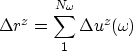 |
(7) |
Equations (6) and (7) establish
a linear relation between the perturbation in slowness
(![]() ) and the perturbation in image (
) and the perturbation in image (![]() ). We can use this
linear relation in an iterative algorithm to invert for the
perturbation in slowness based on the perturbation in the image.
). We can use this
linear relation in an iterative algorithm to invert for the
perturbation in slowness based on the perturbation in the image.