 |
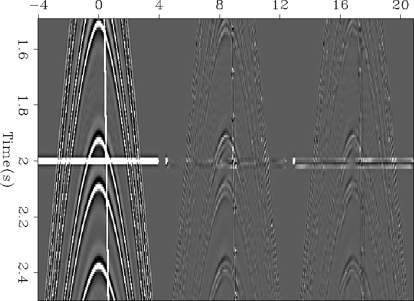
Figure 9 The result after 15 conjugate gradient steps of fitting goals (3). The left panel is the input, the center is using an inverse Laplacian preconditioner, the right panel is using radial smoothing.
integer function npolydiv(adj,add,model,data){
logical                        :: adj,add
real                           :: xx(:),yy(:)
integer                        :: ia, ix, iy, ip
integer, dimension(:), pointer :: lag
real,    dimension(:), pointer :: flt,tt

allocate(tt(size(yy)))
tt = 0.
if( adj) {
        tt = yy
  do iy= nd, 1, -1 { ip = aa%pch( iy)
    lag => aa%hlx( ip)%lag; flt => aa%hlx( ip)%flt
    do ia = 1, size( lag) {
      ix = iy - lag( ia);     if( ix < 1)  cycle
      tt( ix) -=  flt( ia) * tt( iy)
      }
    }
  xx += tt
 } else {
        tt = xx
  do iy= 1, nd { ip = aa%pch( iy)
    lag => aa%hlx( ip)%lag; flt => aa%hlx( ip)%flt
    do ia = 1, size( lag) {
      ix = iy - lag( ia);      if( ix < 1)  cycle
      tt( iy) -=  flt( ia) * tt( ix)
      }
    }
  yy += tt
        }
allocate(tt(size(yy)))
}
PREDICTING A CMP GATHER
To show how radial smoothing can be valuable, we constructed a synthetic CMP gather using a Kirchhoff modeling code. To these CMP gathers we added two lines, one in a radial direction and one at constant time (left panel of Figure 9.) The constant time line can be thought of as noise, while the radial line represents conflicting information that fits our model of valid data.
We then attempted to estimate the shot gather using fitting goals (3) with filters every 20 points in time and every 5 points in offset using two different types of preconditioners. The center panel shows the residual after using an inverse Laplacian Claerbout (1998b) and the right panel, radial smoothers. Generally, the two approaches did approximately the same job in predicting the data. The difference comes where the lines intersect the hyperbolas. If we examine the intersection points, more closely, Figure 10, we see that in the case of the Laplacian we did an equal job of predicting the hyperbolas and the constant time line. When using steering filters, the constant time line is much stronger (we avoid predicting noise).
 |
 |
INTERPOLATING A CMP GATHER
Once filters are estimated, one of their potential uses is missing data interpolation. Systematic gaps in data acquisition may cause data aliasing sufficient to make some processing steps difficult Crawley (1998); Spitz (1991). Adding more traces can dealias the data.
To add more traces, we require that the original data
and the new data have the same dips Claerbout (1997).
The dip information is carried in the PEFs.
The missing data estimation is formulated just like
the filter estimation, except that the PEFs are known and the
data unknown.
Also, we constrain the data by specifying that the originally
recorded traces do not change.
To separate the known and unknown data we have a
known data selector ![]() and an
unknown data selector
and an
unknown data selector ![]() , with
, with ![]() . These multiply by 1 or depending on whether
the data was originally recorded or not.
With
. These multiply by 1 or depending on whether
the data was originally recorded or not.
With ![]() signaling convolution with the PEF and
signaling convolution with the PEF and ![]() the
vector of data, the regression is
the
vector of data, the regression is
![]() , or
, or ![]() .
.
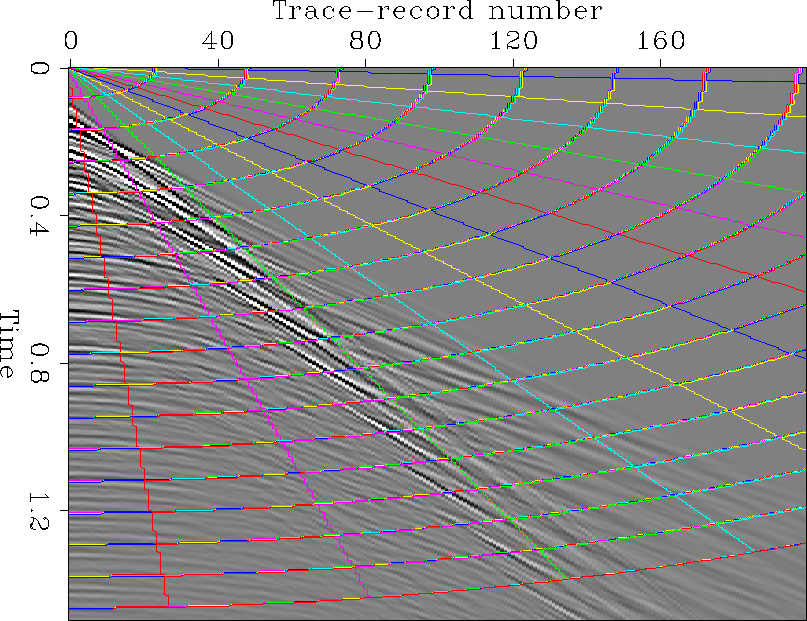
Filters at every data point are cumbersome to estimate, so we estimate filters over small areas. This is just like patching Claerbout (1992d) except that now the patches are not independent. If the patches are independent, there is a lower limit on the patch size, because a patch must contain plenty of data to provide enough fitting equations to determine all the filter coefficients. Experience shows that where the data have curvature, the minimum patch size tends to be too large for the assumption of stationarity to be reasonable. Smoothing the filters allows us to make the patches much smaller, so that stationarity assumptions are workable. We arrange the new patches in polar coordinates, to take advantage of the notion of radial smoothing.
An illustration is given in Figure web.
The cmp gather is overlayed by lines which delineate
patch boundaries.
Degree of smoothing in r and ![]() is adjustable.
The patches shown are fairly large.
Crawley and Claerbout1999 explains further
this method and shows the result of interpolating using radial
patches and smoothers.
is adjustable.
The patches shown are fairly large.
Crawley and Claerbout1999 explains further
this method and shows the result of interpolating using radial
patches and smoothers.
 |