


|
cmpfig
Figure 1 CMP from Mobil AVO data. | 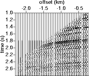 |

Strong surface related multiple energy is characteristic of this region. The main preprocessing steps were hyperbolic Radon filtering and bandpass filtering. The Radon filter suppressed but did not entirely remove coherent noise: it seemed reasonable to hope that primary energy dominates the filtered data, as is required by the dual regularization strategy. The bandpass filter ensured that the data were not spatially aliased, so that the differential semblance could be computed accurately.
Minimization of J0[v;d] produced the RMS velocity displayed in Figure 2, which exhibits a characteristic feature of the differential semblance function: when faced with contradictory moveout (as for example in the interval 1.8-2.4 s), it averages the apparent velocities to come as close as possible to flattening all events. The moveout corrected data (G[v]d in the notation of the last section) displayed in Figure 3 shows a mixture of overcorrected and undercorrected events. The minimization process (via a quasi-Newton algorithm) required approximately 12 s on an SGI Origin2000 processor.
|
sigdisplay0
Figure 2 | 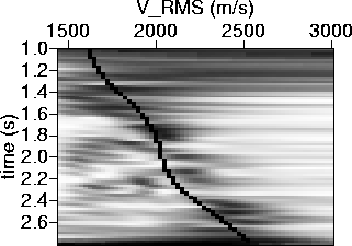 |
|
siginvdata0
Figure 3 Image gather ( = NMO corrected CMP) using | 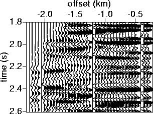 |
We used the output of the J0[v;d] minimization as the initial guess
for minimization of J0.5[v;d]; the latter required approximately
3 min on the Origin. Figure 4 shows that
![]() was not a bad guess at the level of coherent noise: the
automatic velocity analysis has now essentially ignored slow (multiple
reflection) and smaller fast (steeply dipping or out of plane) phases
and placed its estimate of RMS velocity squarely in the main corridor
of apparent primary reflection phases, as one also sees in the the
conventional image gather (= moveout corrected data G[v]d,
Figure 5). Dual regularization also produces an
inverted reflectivity (
was not a bad guess at the level of coherent noise: the
automatic velocity analysis has now essentially ignored slow (multiple
reflection) and smaller fast (steeply dipping or out of plane) phases
and placed its estimate of RMS velocity squarely in the main corridor
of apparent primary reflection phases, as one also sees in the the
conventional image gather (= moveout corrected data G[v]d,
Figure 5). Dual regularization also produces an
inverted reflectivity ( ![]() in the last section,
Figure 6) or denoised data, which is superior to
the conventional image gather as a basis for further processing.
in the last section,
Figure 6) or denoised data, which is superior to
the conventional image gather as a basis for further processing.
|
sigdisplay5
Figure 4 |  |
|
siginvdata5
Figure 5 Image gather ( = NMO corrected CMP) using |  |
|
sigestrefl5
Figure 6 Inverted reflectivity, |  |