 |
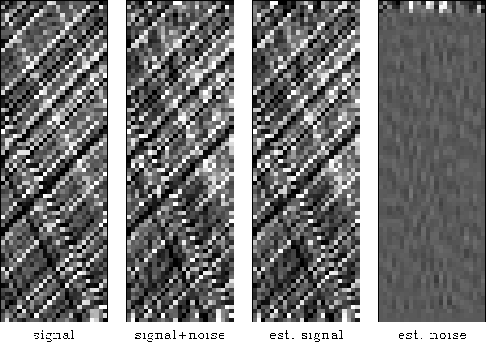
Figure 13 The input signal is on the left. Next is that signal with noise added. Next, for my favorite value of epsilon=1., is the estimated signal and the estimated noise.
Figure 13 demonstrates the concept. I consider the result satisfactory, though I was disappointed that the separation was not ``perfect,'' because the input data is perfect before the noise is added. I was particularly disappointed that the weaker of the two dips is barely recovered, but I believe the code is working according to the theory and that results of about this quality are to be expected.
 |
Various problems occur around the boundaries.
In an effort to avoid these problems,
I experimented with different edge conditions in the convolution.
Best results were found
with transient edge conditions,
when the problem was recast
with the independent variable being ![]() instead of
instead of ![]() .
.
Ray Abma
first noticed that different results were obtained when the
fitting goal was cast in terms of ![]() instead of
instead of ![]() .At first I could not believe his result,
but after repeating the computations independently I had to agree that
the result does depend on the choice of independent variable.
I sought an explanation in terms of differing null spaces,
but this is not yet satisfactory.
.At first I could not believe his result,
but after repeating the computations independently I had to agree that
the result does depend on the choice of independent variable.
I sought an explanation in terms of differing null spaces,
but this is not yet satisfactory.
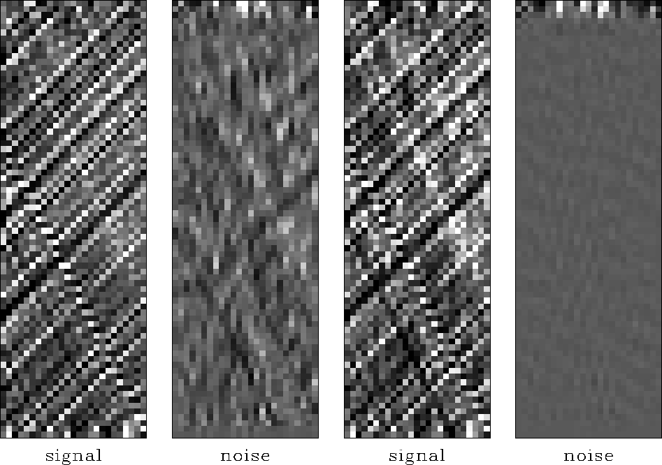
Figure 14 shows the result of experimenting with
the choice of ![]() .As expected, increasing
.As expected, increasing ![]() weakens
weakens ![]() and increases
and increases ![]() .When
.When ![]() is too small,
the noise is small and
the signal is almost the original data.
When
is too small,
the noise is small and
the signal is almost the original data.
When ![]() is too large,
the signal is small and
coherent events are pushed into the noise.
is too large,
the signal is small and
coherent events are pushed into the noise.
 |
 |
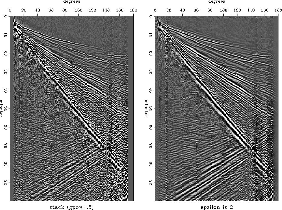
Figure 15 shows a test of noise subtraction by multidip narrow-pass filtering on the Shearer-IDA stack. As with prediction there is a general reduction of the noise. Unlike with prediction, weak events are preserved and noise is subtracted from them too.
Besides the difference in theory,
the separation filters are much smaller
because their size is determined by
the concept that ``two dips will fit anything locally''
(a2=3),
versus the prediction filters
``needing a sizeable window to do statistical averaging.''
The same aspect ratio a1/a2 is kept and
the page is now divided into
11 vertical patches and 24 horizontal patches
(whereas previously the page was divided in ![]() patches).
In both cases the patches overlap about 50%.
In both cases I chose to have about ten times as many equations
as unknowns on each axis in the estimation.
The ten degrees of freedom could be distributed differently
along the two axes, but I saw no reason to do so.
patches).
In both cases the patches overlap about 50%.
In both cases I chose to have about ten times as many equations
as unknowns on each axis in the estimation.
The ten degrees of freedom could be distributed differently
along the two axes, but I saw no reason to do so.