MEANS, MEDIANS, PERCENTILES AND MODES

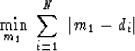
Means, medians, and modes are different averages. Given some data values d_i for i=1,2,...,N, the arithmetic mean value m₂ is

$$m_2 \eq {1 \over N} \ \sum_{i=1}^N \ d_i$$ (1)

It is useful to notice that this m₂ is the solution of the simple fitting problem $d_i \approx m_2$ or $\bold d \approx m_2$,in other words, 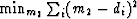$\min_{m_2} \sum_i (m_2-d_i)^2$ or

$$0 \eq {d \over dm_2} \ \sum_{i=1}^N \ (m_2-d_i)^2$$ (2)

The median of the d_i values is found when the values are sorted from smallest to largest and then the value in the middle is selected. The median is delightfully well behaved even if some of your data values happen to be near infinity. Analytically, the median arises from the optimization

$$\min_{m_1}\ \sum_{i=1}^N \ \vert m_1-d_i\vert$$ (3)

To see why, notice that the derivative of the absolute value function is the signum function,

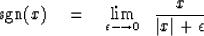$${\rm sgn}(x) \eq \lim_{\epsilon \longrightarrow 0} \ \ { x \over \vert x\vert + \epsilon }$$ (4)

The gradient vanishes at the minimum.

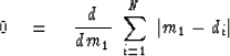$$0 \eq {d \over dm_1} \ \sum_{i=1}^N \ \vert m_1-d_i\vert$$ (5)

The derivative is easy and the result is a sum of sgn() functions,

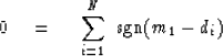$$0 \eq \ \sum_{i=1}^N \ {\rm sgn}(m_1-d_i)$$ (6)

In other words it is a sum of plus and minus ones. If the sum is to vanish, the number of plus ones must equal the number of minus ones. Thus m₁ is greater than half the data values and less than the other half, which is the definition of a median. The mean is said to minimize the L₂ norm of the residual and the median is said to minimize its L₁ norm.

Before this chapter, our model building was all based on the L₂ norm. The median is clearly a good idea for data containing large bursts of noise, but the median is a single value while geophysical models are made from many unknown elements. The L₁ norm offers us the new opportunity to build multiparameter models where the data includes huge bursts of noise.

Yet another average is the ``mode,'' which is the most commonly occurring value. For example, in the number sequence (1,2,3,5,5) the mode is 5 because it occurs the most times. Mathematically, the mode minimizes the zero norm of the residual, namely L₀=|m₀-d_i|⁰. To see why, notice that when we raise a residual to the zero power, the result is 0 if d_i=m₀, and it is 1 if $d_i \ne m_0$.Thus, the L₀ sum of the residuals is the total number of residuals less those for which d_i matches m₀. The minimum of L₀(m) is the mode m=m₀. The zero power function is nondifferentiable at the place of interest so we do not look at the gradient.

 

norms
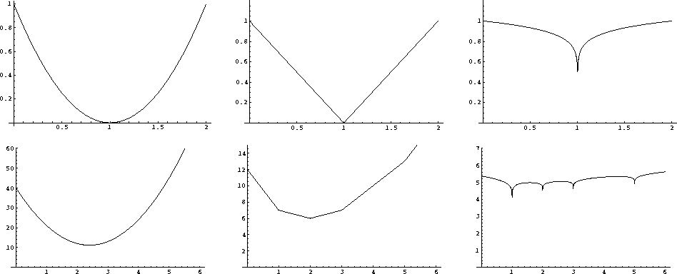
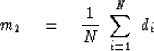
Figure 1 The coordinate is m. Top is the L₂, L₁, and $L_{1/10}\approx L_0$ measures of m-1. Bottom is the same measures of the data set (1,1,2,3,5).

L₂(m) and L₁(m) are convex functions of m (positive second derivative for all m), and this fact leads to the triangle inequalities 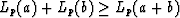$L_p(a)+L_p(b) \ge L_p(a+b)$ for $p\ge 1$and assures slopes lead to a unique (if p>1) bottom. Because there is no triangle inequality for L₀, it should not be called a ``norm'' but a ``measure.''

Because most values are at the mode, the mode is where a probability function is maximum. The mode occurs with the maximum likelihood. It is awkward to contemplate the mode for floating-point values where the probability is minuscule (and irrelevant) that any two values are identical. A more natural concept is to think of the mode as the bin containing the most values.