|
subsine390
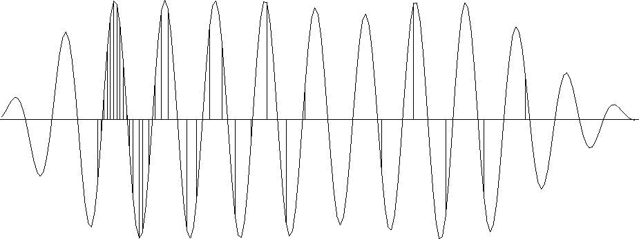
Figure 14 Interpolating with a three-term filter. The interpolated signal is fairly monofrequency. |  |
![[*]](http://sepwww.stanford.edu/latex2html/cross_ref_motif.gif) and
and
![[*]](http://sepwww.stanford.edu/latex2html/cross_ref_motif.gif) .
What is new here is that the proper PEF
is not given but is determined from the data.
Figure 14 was made with a three-coefficient filter (1,a1,a2) and
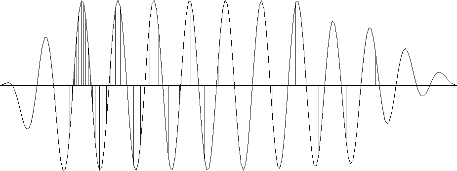
Figure 15 was made with a five-coefficient filter
(1,a1,a2,a3,a4).
The main difference in the figures is where the data is sparse.
The three-coefficient filter can fit only a single sinusoid and it does that.
The five-coefficient filter can fit only two sinusoids and
it does something like that, a high-frequency sinusoid on the left
and a lower one on the right.
The data points in Figures
.
What is new here is that the proper PEF
is not given but is determined from the data.
Figure 14 was made with a three-coefficient filter (1,a1,a2) and
Figure 15 was made with a five-coefficient filter
(1,a1,a2,a3,a4).
The main difference in the figures is where the data is sparse.
The three-coefficient filter can fit only a single sinusoid and it does that.
The five-coefficient filter can fit only two sinusoids and
it does something like that, a high-frequency sinusoid on the left
and a lower one on the right.
The data points in Figures
![[*]](http://sepwww.stanford.edu/latex2html/cross_ref_motif.gif) ,
14 and
15 are samples from a sinusoid.
,
14 and
15 are samples from a sinusoid.
|
subsine390
Figure 14 Interpolating with a three-term filter. The interpolated signal is fairly monofrequency. |  |
|
subsine590
Figure 15 Interpolating with a five term filter. A low frequency component grows towards the right. |  |
|
Comparing Figures
|