Adjoint derivative

Given a sampled signal, its time derivative can be estimated by convolution with the filter $(1,-1)/\Delta t$,expressed as the matrix-multiply below:  

$$\left[ \begin{array} {c} y_1 \\ y_2 \\ y_3 \\ y_4 \\ y_... ..._1 \\ x_2 \\ x_3 \\ x_4 \\ x_5 \\ x_6 \end{array} \right]$$ (3)

The filter impulse response is seen in any column in the middle of the matrix, namely (1,-1). In the transposed matrix, the filter-impulse response is time-reversed to (-1,1). So, mathematically, we can say that the adjoint of the time derivative operation is the negative time derivative. This corresponds also to the fact that the complex conjugate of $-i\omega$ is $i\omega$.We can also speak of the adjoint of the boundary conditions: we might say that the adjoint of ``no boundary condition'' is a ``specified value'' boundary condition.

A complicated way to think about the adjoint of equation (3) is to note that it is the negative of the derivative and that something must be done about the ends. A simpler way to think about it is to apply the idea that the adjoint of a sum of N terms is a collection of N assignments. This is done in module igrad1, which implements equation (3) and its adjoint. The last row in equation (3) is optional and depends not on the code shown, but the code that invokes it. It may seem unnatural to append a null row, but it can be a small convenience (when plotting) to have the input and output be the same size.  

module igrad1 {	                                   # gradient in one dimension
#%  _lop( xx,  yy)
integer i
do i= 1, size(xx)-1 {
        if( adj) {
                xx(i+1) = xx(i+1) + yy(i)
                xx(i  ) = xx(i  ) - yy(i)
		}
	else
                yy(i) = yy(i) + xx(i+1) - xx(i)
	}
}

The do loop over i assures that all values of yy(i) are used, whether computing all the outputs for the operator itself, or in the adjoint, using all the inputs. In switching from operator to adjoint, the outputs switch to inputs. The Loptran dialect allows us to write the inner code of the igrad1 module more simply and symmetrically using the syntax of C, C++, and Java. Expressions like a=a+b can be written more tersely as a+=b. With this, the heart of module igrad1 becomes

if( adj) {   xx(i+1) += yy(i)
             xx(i)   -= yy(i)
           }
else {       yy(i)   += xx(i+1)
             yy(i)   -= xx(i)
           }

where we see that each component of the matrix is handled both by the operator and the adjoint. Think about the forward operator ``pulling'' a sum into yy(i), and think about the adjoint operator ``pushing'' or ``spraying'' the impulse yy(i) back into xx(). Something odd happens at the ends of the adjoint only if we take the perspective that the adjoint should have been computed one component at a time instead of all together. By not taking that view, we avoid that confusion.

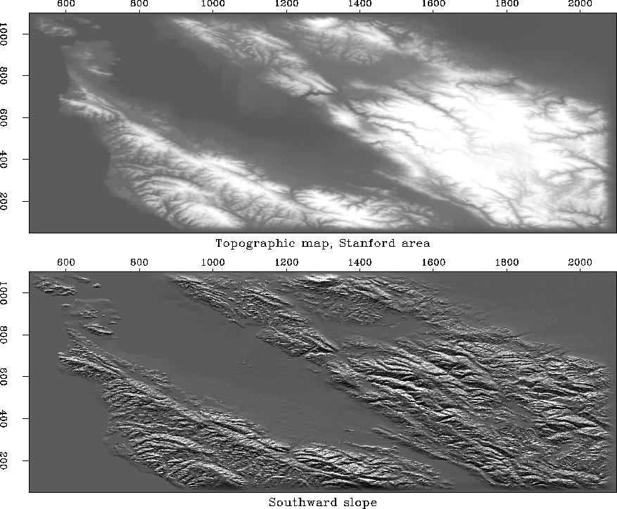
Figure stangrad90 illustrates the use of module igrad1 for each north-south line of a topographic map. We observe that the gradient gives an impression of illumination from a low sun angle.

 

stangrad90
Figure 1 Topography near Stanford (top) southward slope (bottom).

To apply igrad1 along the 1-axis for each point on the 2-axis of a two-dimensional map, we use the loop

do iy=1,ny
      stat = igrad1_lop (.false., .false., map(:,iy), ruf(:,iy))

On the other hand, to see the east-west gradient, we use the loop

do ix=1,nx 
      stat = igrad1_lop (.false., .false., map(ix,:), ruf(ix,:))