Modeling ocean-bottom seismic rotation rates

Modeling results

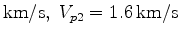
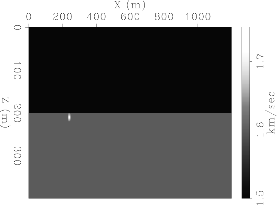
The purpose of the modeling we ran was to synthesize ocean-bottom seismic acquisition, therefore we used a simple 2-layer model of water over solid. The source was at the water surface, and receivers were at the water bottom. We executed two runs: one with a near-seabed anomaly, and one without. The anomaly generated scattering of both P and S waves, which upon interacting with the seabed also gave rise to a seabed interface wave. The model without the anomaly enabled us to see which part of the wavefield was due to the scattering. The $V_p$ velocity models used are shown in Figures 3(a) and 3(b). The parameters of the two layers were:

1. $V_{p1} = 1.5 \,$$\text {km}/\text s, \; V_{p2} = 1.6 \, \text {km}/\text s$ .
2. $V_{s1} = 0 \,$$\text {km}/\text s, \; V_{s2} = 0.6 \, \text {km}/\text s$ .
3. $\rho_1 = 1.025 \,$$\text {gr}/\text {cm}^3, \; \rho_2 = 1.7 \, \text {gr}/\text {cm}^3$ .

The anomaly was a Gaussian, which extended outward to a radius of 10 meters, and was centered 10 meters below the seabed. The medium parameters at the center of the anomaly were: $V_p = 1.75 \,$$\text {km} / \text s$ , $V_s = 0.9 \,$$\text {km}\text s$ , and $\rho = 2.1 \,$$\text {gr} / \text {cm}^3$ . We did not do any testing with the anomaly parameters, although presumably altering these parameters would result in greater or lesser scattering. At this point, all we required was a feasible source of surface waves. A near-seabed anomaly simulates a ``rock'' buried just below the seabed, or the leg of a platform, either of which could be sources for scattered surface waves. Our source was a pressure source simulating an airgun, located at the water surface. The wavelet was a Ricker with $25$Hz central frequency. There is no source-side ghost from the water surface, since we used an absorbing upper boundary. However, this ghost is simulated by the second lobe of the injected Ricker wavelet.

vp2d,vp2d-anom
Figure 3. P-wave velocity models. (a) velocity model without anomaly. (b) velocity model with anomaly. The anomaly is a Gaussian, with a diameter of 20 meters.

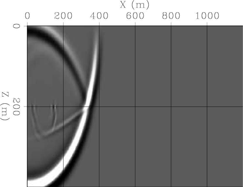
Figures 4(a) and 4(b) are snapshots of the vertical and horizontal P particle velocities of the entire wavefield at $t=0.3$$\text s$ . The incident, reflected and transmitted P-waves are prominent in these snapshots. Also visible is the transmitted S-wave, which is the conversion of the P-wave inciding on the seabed. The scattered S-wave and Scholte wave are visible as a semicircle, expanding from the anomaly location at $x=100$$\text m$ .

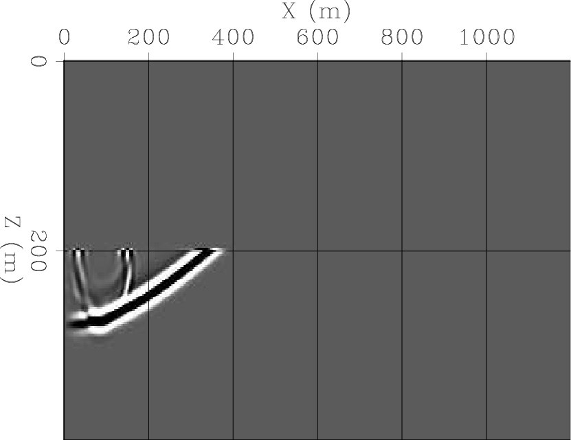
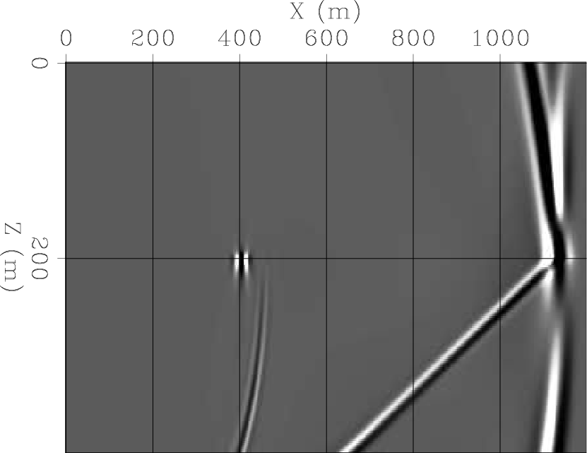
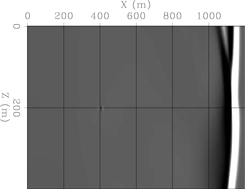
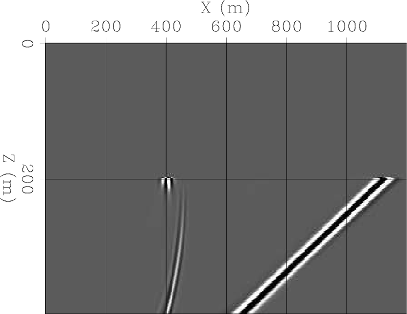
Figure 4(c) is the pressure as calculated by equation 3. We can see that the waves that generate most of the volumetric deformation are indeed the P-waves. However, the Scholte wave also generates some volumetric deformation at the seabed. Figure 4(d) is the rotation as calculated by equation 4. The waves that generate shear deformation (and thus rotational motion at the surface) are the transmitted S-wave, and the scattered S and Scholte waves. Notice that the transmitted S-wave is coming off the P head-wave, and is therefore propagating along the seabed at P-wave velocity.

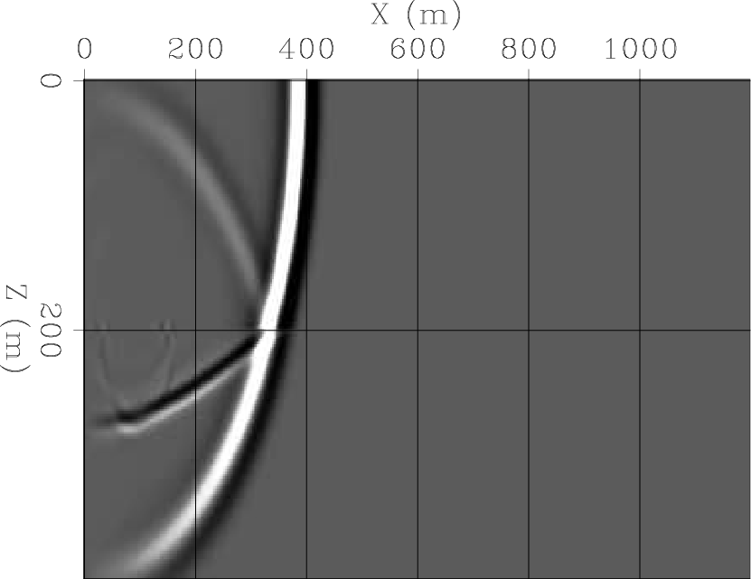
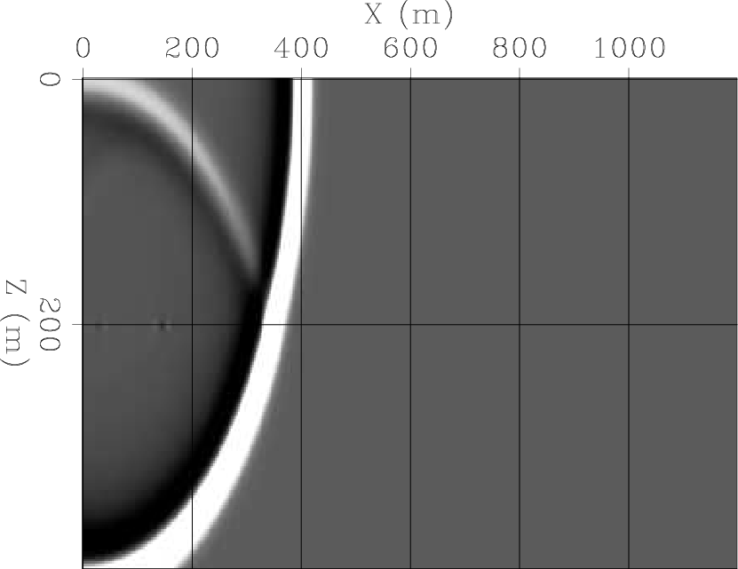
Figures 5(a)-5(d) are snapshots of the same four fields, at $t=0.8$$\text s$ . The scattered S-wave and the scattered Scholte wave are separated at this point in the propagation, since the velocity of surface waves is slightly lower than that of S-waves. The imprint of the Scholte wave on both the pressure and the rotation sections is visible.

0vx2b,0vz2b,0P2b,0rot2b
Figure 4. Wavefield snapshots at $t=0.3$$\text s$ seconds for the velocity model containing a near-surface anomaly. (a) Vertical particle velocity. (b) Horizontal particle velocity. (c) Pressure. (d) Rotation. The source is an airgun near the sea surface. In (a) and (b), all wave modes are present: direct P, reflected P, transmitted P and transmitted S. Also apparent are the S and Scholte waves which have scattered off the anomaly at $x=100m$ . In (c) and (d) there is separation: the S waves are not in (c) and P waves are not in (d). The surface waves are in both (c) and (d).

0vx2,0vz2,0P2,0rot2
Figure 5. Wavefield snapshots at $t=0.8$ seconds for the velocity model containing a near-surface anomaly. (a) Vertical particle velocity. (b) Horizontal particle velocity. (c) Pressure. (d) Rotation. Note how the scattered S body wave and the Scholte surface wave separate with travel time, as a result of their slightly differing velocities. Note that the Scholte wave generates both a rotational and a volumetric deformation.

Figures 6(a) and 6(b) are the vertical and horizontal particle displacement recordings at the seabed for the velocity model without the anomaly. Figures 6(c) and 6(d) are the pressure and rotation, respectively. The incident P-wave causes both a pressure deformation and a shear deformation at the surface, and it therefore generates a transmitted S-wave. However the moveout of the S-wave is still that of the P-wave.

0uxr1,0uzr1,0Pr1,0rotr1
Figure 6. Synthetic data recording at sea-bottom without anomaly. (a) Vertical particle displacement. (b) Horizontal particle displacement. (c) Pressure. (d) Rotation.

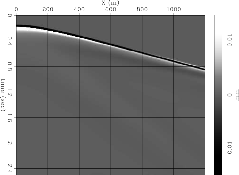
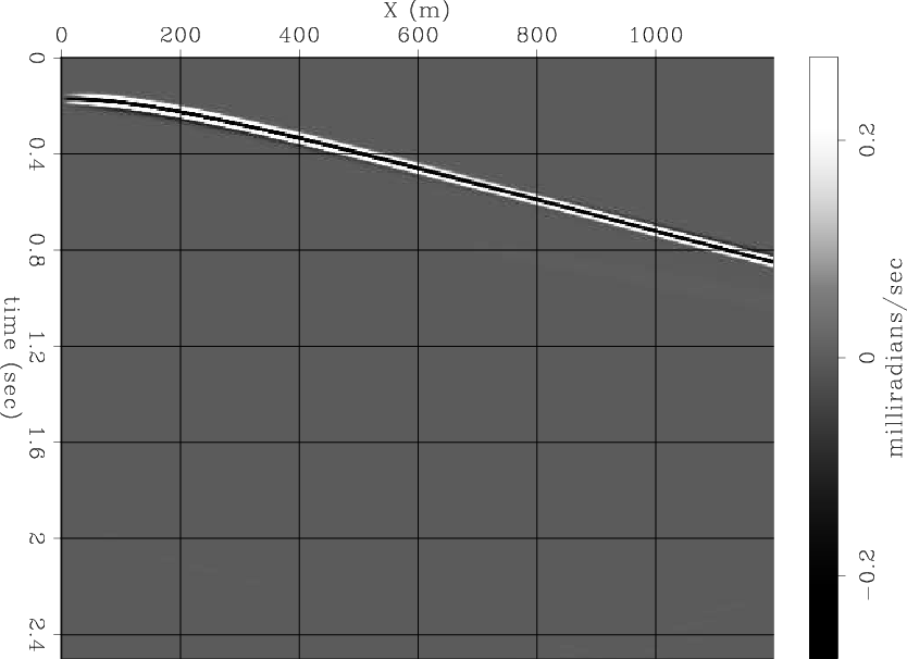
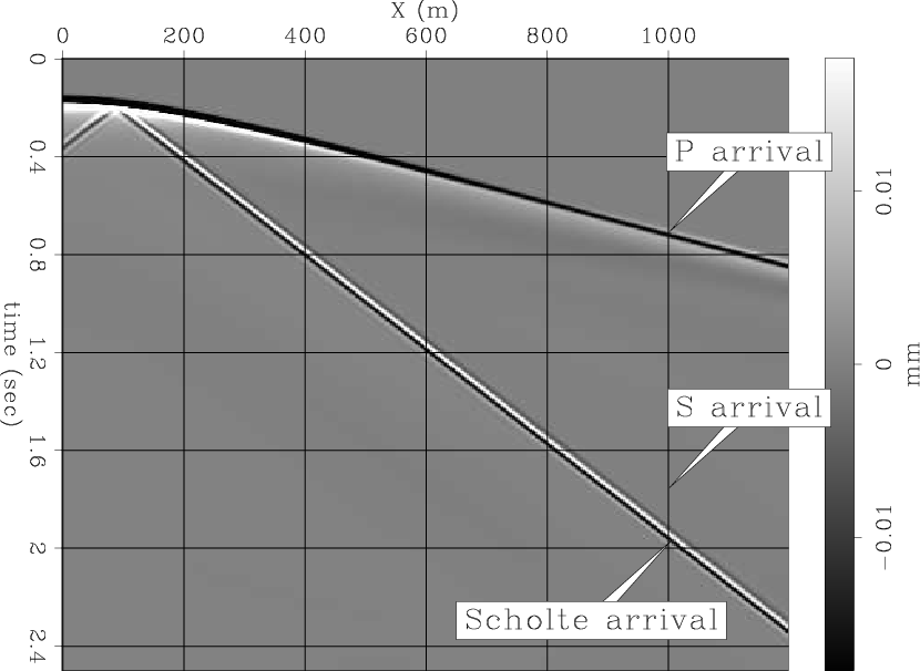
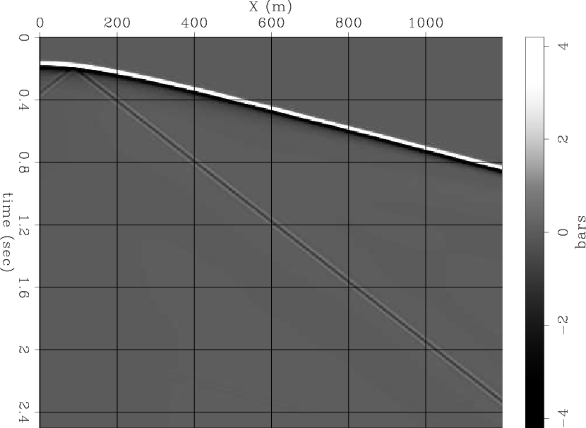
Figures 7(a) and 7(b) are the vertical and horizontal particle displacement recordings at the seabed for the velocity model containing the anomaly. At $x=1000$$\text m$ , the arrivals of the direct P, scattered S and scattered Scholte wave are are marked. The S arrival is too weak compared to the P and Scholte waves to be observed in these sections. Figures 7(c) and 7(d) are the pressure and rotation recordings. We can think of these sections as the hydrophone and rotational sensor recordings. Comparing Figures 6(d) and 7(d), we can see that while most of the linear particle displacement is due to the P-wave, the Scholte wave is responsible for generating strong rotational motion.

0uxr2,0uzr2,0Pr2,0rotr2
Figure 7. Synthetic data recording at sea-bottom with anomaly. The scattered Scholte wave is visible, but the scattered S-wave is relatively too weak to observe in these sections. The annotations indicate where time windows were taken for the plots in the next figure. (a) Vertical particle displacement. (b) Horizontal particle displacement. (c) Pressure. (d) Rotation.

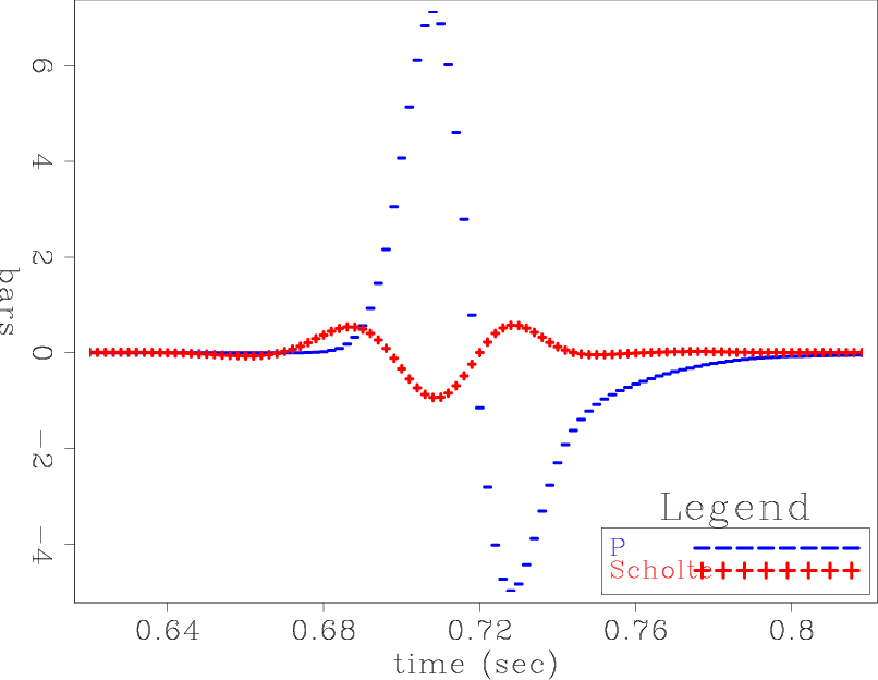
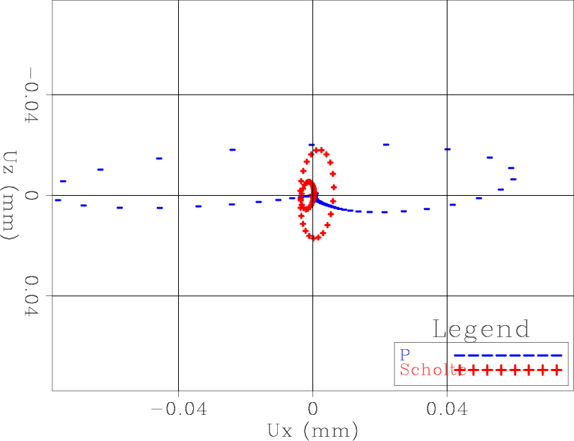
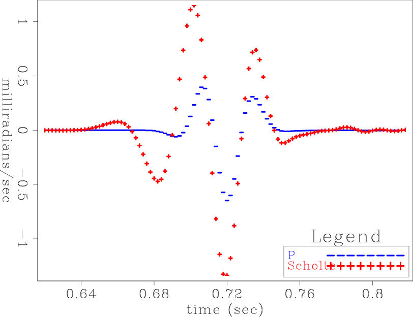
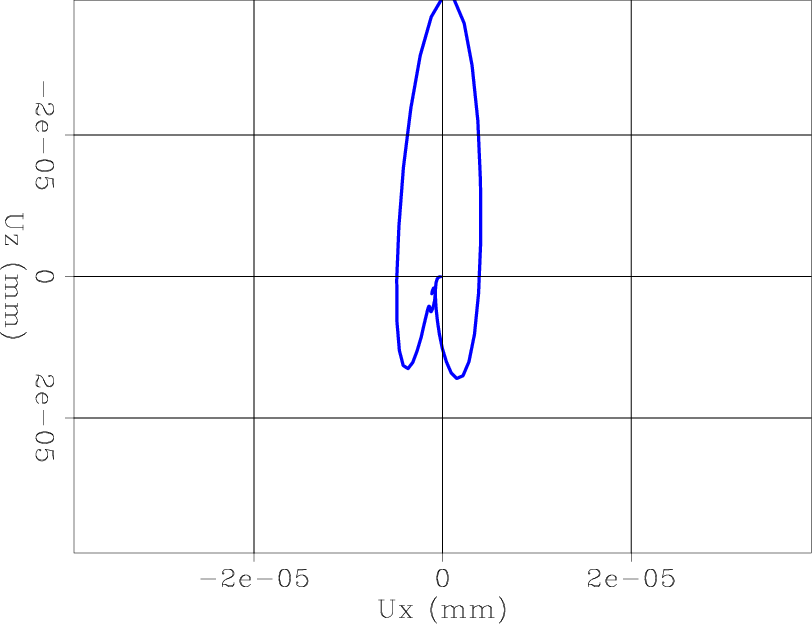
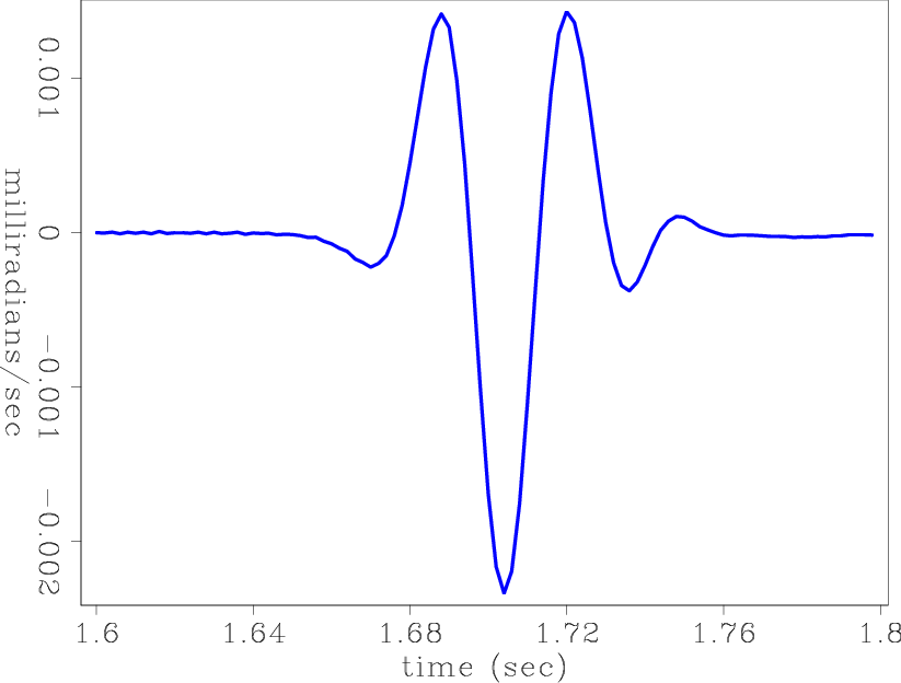
Figures 8(a)-9(c) show the three separate arrival-time windows of each wave type. The arrival times and offset where they were extracted from are marked in Figure 7(a). Figure 8(a) is the volumetric pressure generated by the P-wave and Scholte wave arrivals, as calculated by equation 3. Figure 8(b) is the hodogram of particle displacements of those arrivals. Notice that the P hodogram is slightly elliptical, which means that the particle motion is not linear, as it is in a body wave. The reason for that is the mode conversion which takes place when the P-wave hits the seabed. What we are seeing is a combination of P and S displacements. We can see however that the Scholte displacement hodogram is very elliptical. Figure 8(c) is the rotation rate of the P and Scholte arrivals, as calculated by equation 4. The P-wave does generate some rotational motion, and this is again a result of the mode conversion at the seabed. However, the Scholte wave generates greater rotational motion, even though the linear displacements of this wave are much weaker than those of the P-wave.

Figures 9(a)-9(c) are the pressure, displacement hodogram and rotation rate of the scattered S-wave arrival. The volumetric pressure this arrival generates is very weak compared to the P-wave, but while its displacements are 3 orders of magnitude weaker than those of the P-wave, its rotational motion is only 2 orders of magnitude weaker. Note how the hodogram is nearly perpendicular to the P-wave displacement hodogram.

0Pr2-p-gr,0uxzr2-p-gr-hodo,0rotr2-p-gr
Figure 8. P and Scholte wave arrivals at the ocean-bottom receiver at $x=1000m$ , where the scattering was off the anomaly. (a) Pressure of arrivals. (b) Hodogram of displacements of arrivals. (c) Rotation rate of arrivals. Note how the P-wave has greater linear displacements compared to the Scholte wave, but a smaller rotation rate.

0Pr2-s,0uxzr2-s-hodo,0rotr2-s
Figure 9. Shear wave arrival at the ocean-bottom receiver at $x=1000m$ , where the scattering was off the anomaly. (a) Pressure of S arrival. (b) Hodogram of displacements of S arrival. (c) Rotation rate of S arrival.

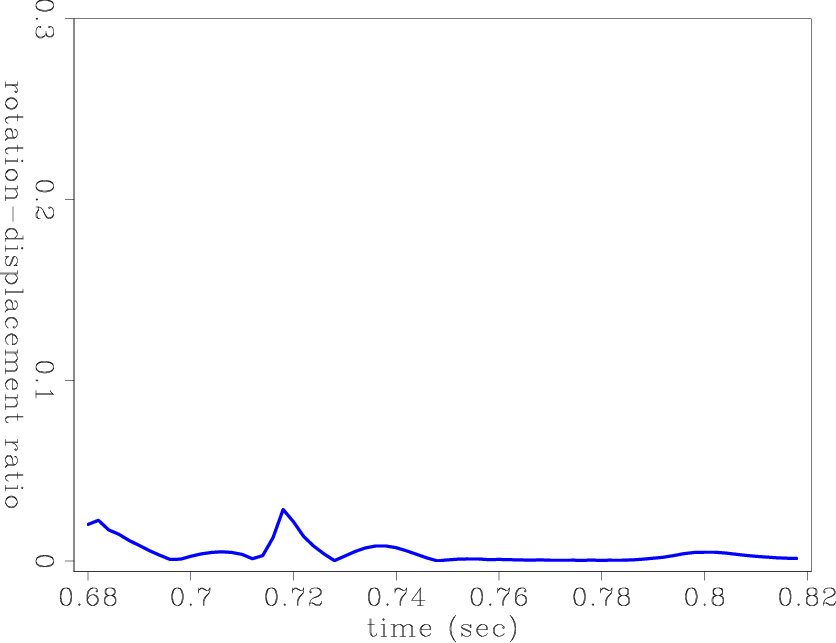
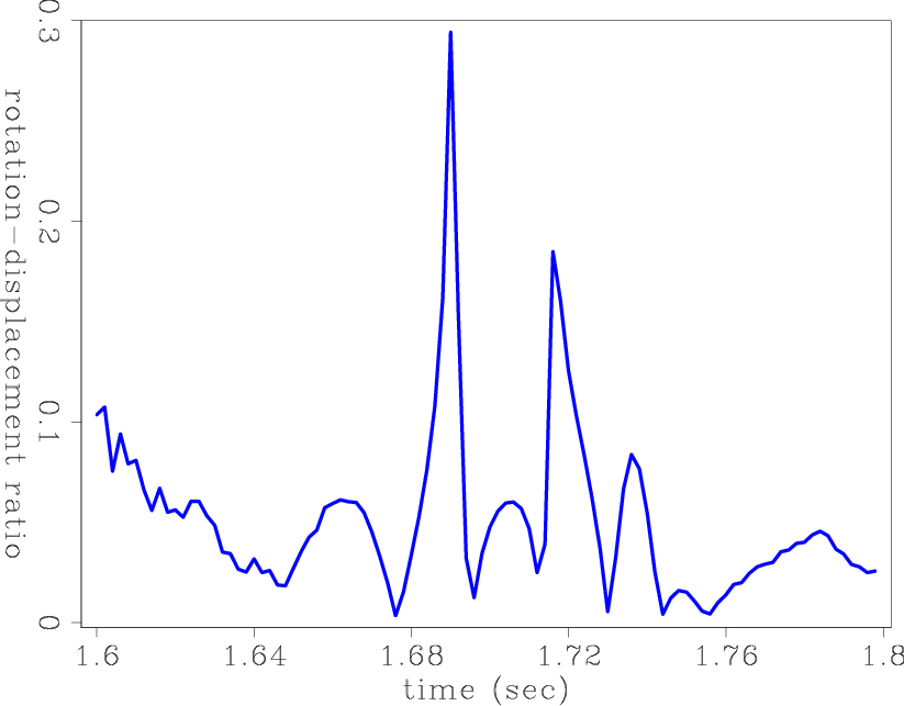
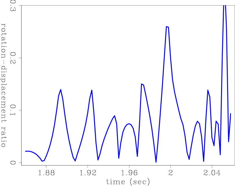
Figures 10(a),10(b) and 10(c) are the ratios between the rotation rates and the absolute value of the displacement vectors of the P, S and Scholte wave arrivals. This ratio serves as a good indication as to which of the waves is a P-wave, and which are S or Scholte waves. The S and Scholte waves give rise to much more rotational motion in comparison to linear motion. P-waves, even when propagating along the seabed, generate mostly linear particle motion.

0rotind2-p,0rotind2-s,0rotind2-gr
Figure 10. Ratio of rotation rate to absolute value of displacement for P, S and Scholte wave arrivals at the ocean-bottom receiver at $x=1000$$\text m$ , where the scattering was off the anomaly. (a) Ratio for P arrival. (b) Ratio for S arrival. (c) Ratio for Scholte wave arrival. Note that the ratio for S and Scholte waves is an order of magnitude greater than for the P wave.

Modeling ocean-bottom seismic rotation rates