Single frequency 2D acoustic full waveform inversion

Time-domain kernel

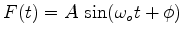We seek to compute solutions of equation 1 for single frequencies. Thus assume that we have a time domain source function acting at a single frequency $F(t) = A\ \mathrm{sin}(\omega_o t + \phi)$ . In a 2D acoustic system this would excite a wave equation as

$$\left( \nabla^2 + v^{-2}(\omega_o,\mathbf x)\partial^2_t \right) d(t,\mathbf{x}) = A(\mathbf{x})\ \mathrm{cos}(\omega_o t - \phi(\mathbf{x}) ),$$ (2)

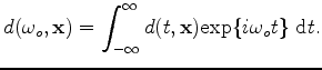
The phase and amplitude of the solution, $V(\omega,\mathbf{x})$ , at frequency $\omega_0$ is simply computed with a forward Fourier transform

$$d(\omega_o,\mathbf{x}) = \int_{-\infty}^{\infty} d(t,\mathbf{x}) \mathrm{exp}\{ i\omega_o t\} \ \mathrm{d}t.$$ (3)

If the solution of 2 is computed accurately, then $d(\omega,\mathbf{x})=0$ for $\omega\neq\pm\omega_o$ . The sourcing terms $A(\mathbf{x})$ and $\phi(\mathbf{x})$ are only non zero where sources act.

To evaluate this inverse Fourier transform, we would need to perform infinite number of time steps and at minus infinity, practically impossible. However, the solution is periodic, thus we can suffice with having computed the wave field for as little as one period. However, we need to initialize the wave field first and wait for the energy of the source to have spread throughout the medium. The computational boundaries could be made absorbing, but this is a challenge, especially at the longer wavelengths that we are interested in modelling. A simpler solution is to extend the domain and omit updating the boundaries. The domain has to be extended large enough to avoid reflections to start modulating the phase throughout the inner area of the model domain that is of interest. This requires a much larger model space, but keeps coding simple and stable.

The kernel is started and run for enough time steps to have the energy of one period to propagate beyond all receivers, assuming one period is enough to stabilize the amplitude and phase of the wave field. This propagation time length is based on a minimum velocity. Then the code steps through two periods while the receiver wave field is kept. We do not need to have a memory variable for the source function or to collect the wave field at the receiver locations. Instead, we upload one sinusoid with a phase from -1$\pi$ to 3.5$\pi$ . A simple $mod$ function statement reduces any absolute phase to fall within that range. The value for a sinusoid with a phase shift of up to $\pm\pi$ can easily be retrieved. And similarly the value of a cosine is available though a shift of $.5\pi$ . The discrete inverse Fourier transform is performed on the fly. No memory transfer needs to occur between CPU and GPU while the modelling is running through the time steps.

An upside of this algorithm is that is is embarrassingly parallel over shots and frequencies, not memory intensive and boundary conditions can be neglected. The downside of this approach is that each frequency inversion requires solving a time-domain waveform inversion, hence this approach is suboptimal and is only implemented here because of the straightforward implementation on CUDA of the 2D waveform inversion with the special excitation source 15. An alternative approach to this problem is to solve the waveform inversion for equation 1 in the frequency domain using a Helmhotz solver that lends itself to efficient CUDA implementation.

Single frequency 2D acoustic full waveform inversion