|
|
|
|
Single frequency 2D acoustic full waveform inversion |
 from observed solutions to our postulated surface wave propagation equation 1 in the frequency domain, where
  is an arbitrary excitation source waveform. As has been noted above, 2D waveform inversion can be directly applied to this problem, with the only exception that inversion results for individual frequencies are treated as separate values of the frequency-dependent velocity
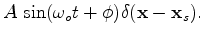
and not applied in a multi-scale velocity refinement of the standard for the waveform inversion process. While the applicability of 2D the waveform inversion is conceptually obvious, technical challenges arise in adapting specific implementations of the waveform inversion to equation 2. Our time domain CUDA implementation of the 2D acoustic equation solves equation 2 with an excitation source of the form
. First, Fourier-transforming 2, we can see that recovering the velocity from a solution to 2 with the source 15 is equivalent to recovering the velocity from a solution to
is an arbitrary excitation source waveform. As has been noted above, 2D waveform inversion can be directly applied to this problem, with the only exception that inversion results for individual frequencies are treated as separate values of the frequency-dependent velocity
and not applied in a multi-scale velocity refinement of the standard for the waveform inversion process. While the applicability of 2D the waveform inversion is conceptually obvious, technical challenges arise in adapting specific implementations of the waveform inversion to equation 2. Our time domain CUDA implementation of the 2D acoustic equation solves equation 2 with an excitation source of the form
. First, Fourier-transforming 2, we can see that recovering the velocity from a solution to 2 with the source 15 is equivalent to recovering the velocity from a solution to
 we get
![$\displaystyle \frac{A}{2}\left[ \delta(\omega-\omega_0)+\delta(\omega+\omega_0) \right]$](img56.png)
in the right-hand side of 16. Now assuming that the velocity is an even function of the frequency, and that we attempt to reconstruct the velocity from 2 with
 , we can see from equation 16 that we can equivalently run 2D waveform inversion 2 for frequencies
![$ \omega \in [0,Nyq]$](img58.png) with
with
 in 15. For an odd waveform (but still even velocity) for each
  we use
 . An arbitrary waveform can be represented as the sum of an even and odd components, and equation 2 will have a linear combination of two source terms 15 in the right-hand side.
|
|
|
|
Single frequency 2D acoustic full waveform inversion |
![$\displaystyle \Delta u + \frac{\omega^2 u}{c^2}=\frac{A}{2 i}\left[ e^{i \phi}\delta(\omega-\omega_0)-e^{-i\phi}\delta(\omega+\omega_0)\right].$](img54.png)