Continuous monitoring by ambient-seismic noise tomography

Passive seismic interferometry

To perform passive seismic interferometry, we cross-correlate passive seismic recordings between all possible station pairs in a permanently installed array. This creates a full virtual seismic survey, $\mathbf{D}(\omega)=\mathrm{D}(\omega,x_r,x_s)$ :

$$\mathbf{D}(\omega) = \mathbf{r}(\omega)\ \mathbf{r}(\omega)^\dag ,$$ (1)

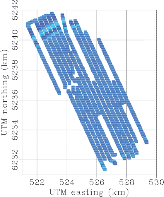
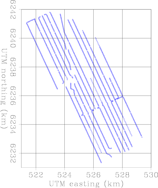
where $\mathbf{r}(\omega)=\mathrm{r}(\omega,x)$ is a vector containing passive seismic recordings at all stations, and $\dag$ denotes the Hermitian (complex conjugation and transposition). However, this technique holds only when the energy in the ambient seismic field satisfies a condition known as energy equipartitioning. In practice, this requirement limits the application of seismic interferometry to certain frequency regimes. The ambient seismic field at low frequencies (0.18 - 1.75 Hz) is dominated by the double-frequency microseism peak, a source of seismic energy that satisfies the requirement of energy equipartition and can be utilized for seismic interferometry (Stewart, 2006; Dellinger and Yu, 2009). At the Valhall oil field, this microseism energy is recorded by the aforementioned permanent installed seismic array (see station map in Figure 1). The microseism energy recorded by the vertical component of the OBC consists of excitations of the Scholte-wave mode of the seafloor.

xy-joseph Figure 1. Station map of OCB at Valhall.

These installations are capable of making recordings continuously for long periods and under all weather conditions. One such recording was made in December 2010, spanning a little over 5 days. Figure 2 shows how the spectrum of the ambient seismic field, as recorded far away from the platform, changes over time. The spectrum is computed over 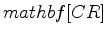$2.5$  minute overlapping windows and averaged over several receivers far removed from the platform. Clearly the microseism energy strength varies over time. Figure 3 contains recordings of wave height and wind strength made at Ekofisk (NMI, 2012), another oil-field near Valhall. Although the weather station is at $32$  km from Valhall, there is a clear correlation between the strength of the microseism energy and the wind strength. This corroborates atmosphere-ocean-seafloor coupling as the source of this microseism energy (Rhie and Romanowicz, 2004,2006; Longuet-Higgins, 1950).

joseph-spectra-low
Figure 2. Spectrum of the ambient seismic field, computed over $2.5$  minute overlapping windows. The spectrum is averaged over several receivers far removed from the platform and displayed as a function of time.

weather
Figure 3. Wind-speed and wave-height measurements at Ekofisk, another oil field near the Valhall field (NMI, 2012).

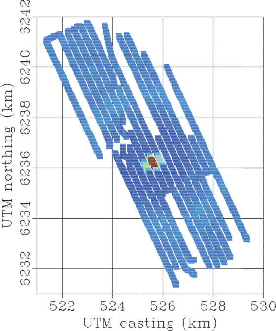
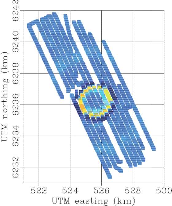
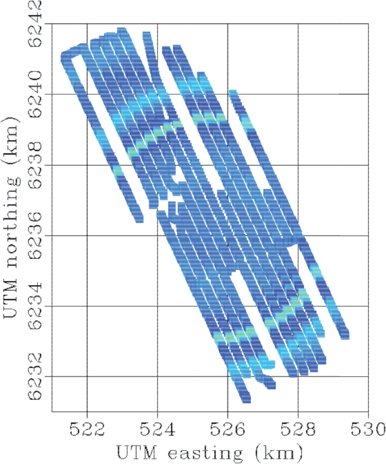
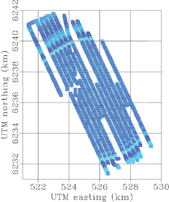
An example of a virtual source is shown in Figure 4. This is one column in the matrix $\mathbf{D}$ , for which all data are cross-correlated with the data at a station in the center of the array. Six time slices are shown, at 0 , $3$ , $6$ , $9$ , $12$ and $15$ seconds. Although the energy focuses at the source at $t=0$ seconds, there is energy at $t=0$ in the vicinity of the master station because the virtual source is finite in bandwidth and zero phase. The wavefront is dispersive: lower frequencies propagate faster the higher frequencies. The virtual source radiates very homogeneously in all directions, reflecting that the energy in the ambient seismic field, averaged over 5 days, was travelling in about equal strength in all directions. The dispersion in the virtual sources can be made visible by transforming the virtual sources from the $(t,x)$ domain to the $(\omega,p)$ domain and stacking all virtual sources in one line of the Valhall array together. The dispersion image is shown in Figure 5. For most of the frequency range, the virtual sources are dominated by a single dispersive wave mode.

frame0s,frame3s,frame6s,frame9s,frame12s,frame15s
Figure 4. A virtual seismic source located in the center of the array. Time slices at: 0 (a), 3 (b), 6 (c), 9 (d), 12 (e) and 15 seconds (f).

Laura-VV-SI-wpLL
Figure 5. Dispersion image for virtual seismic sources in one OBC line of the array. The virtual sources are dominated by a single, dispersive wave mode.

Continuous monitoring by ambient-seismic noise tomography