Recent progress regarding logarithmic Fourier-domain bidirectional deconvolution

Synthetic data example for gain function

In real field data, there usually is an amplitude decay with time. This can be caused by geometric divergence and other factors. The larger the amplitude in the data, the larger the residual. Therefore, the deconvolution will honor early data more than later data. Hence we need a gain function in the deconvolution to boost the contribution of later data.

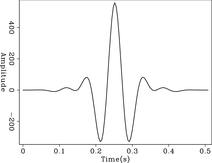
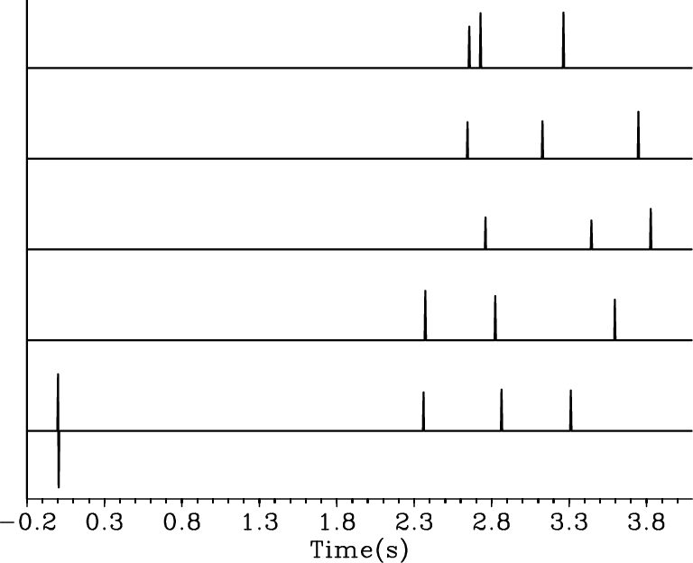
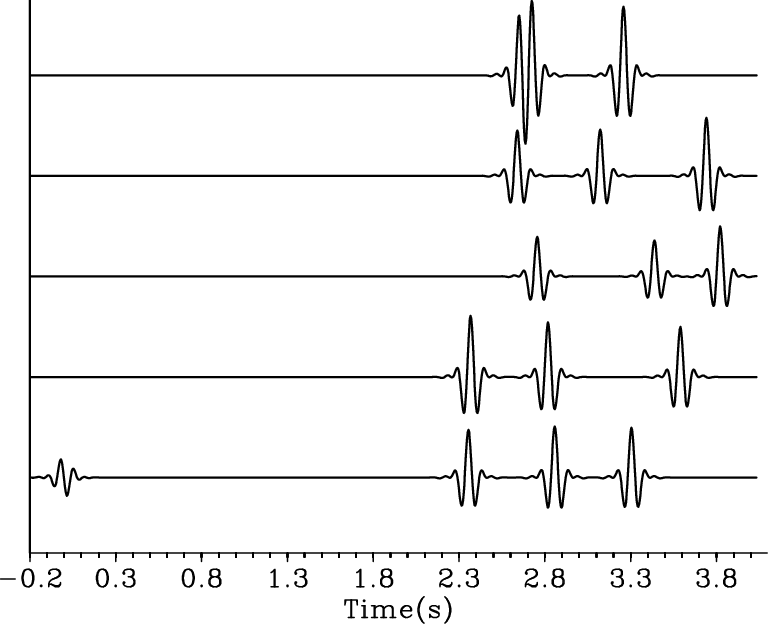
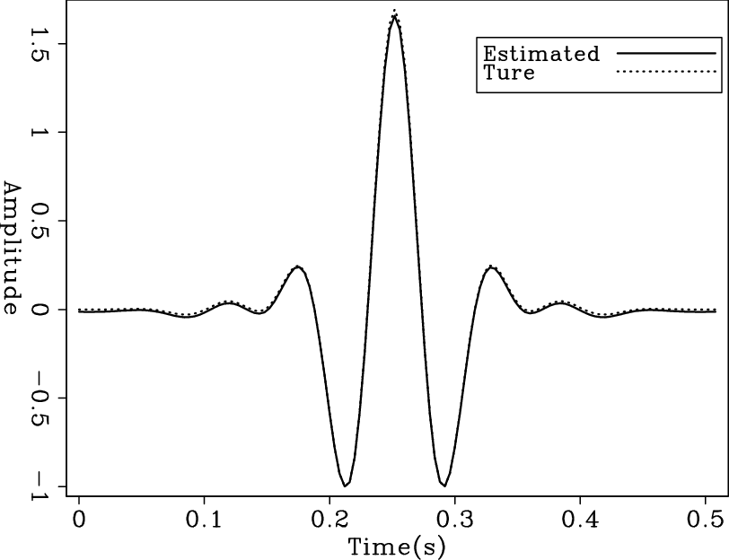
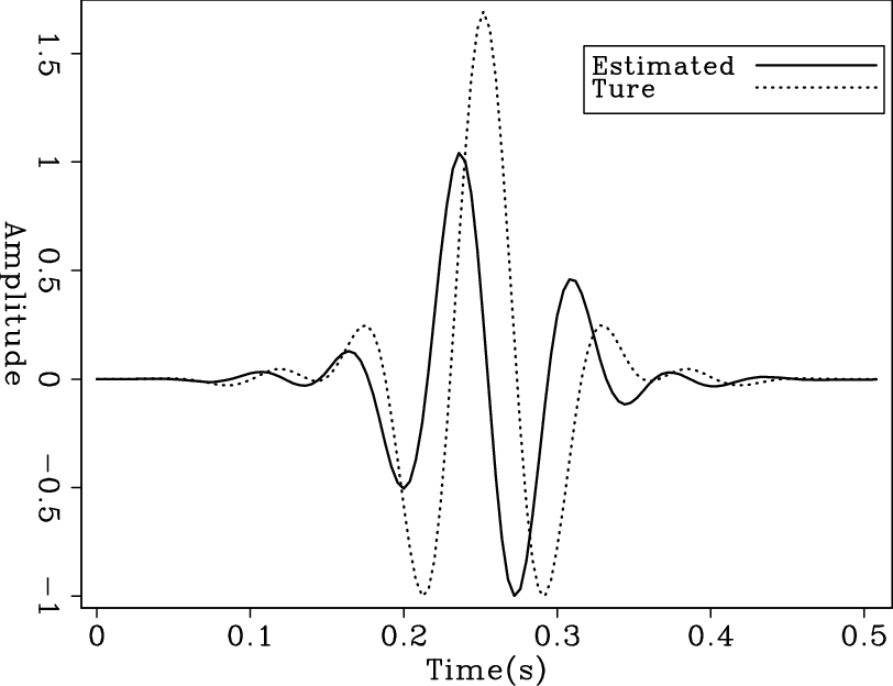
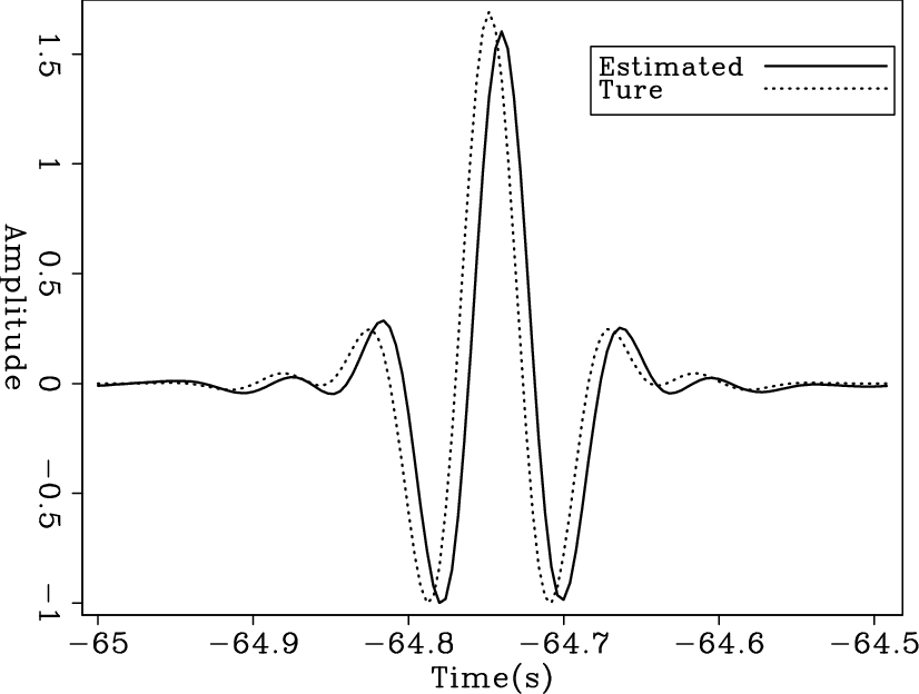
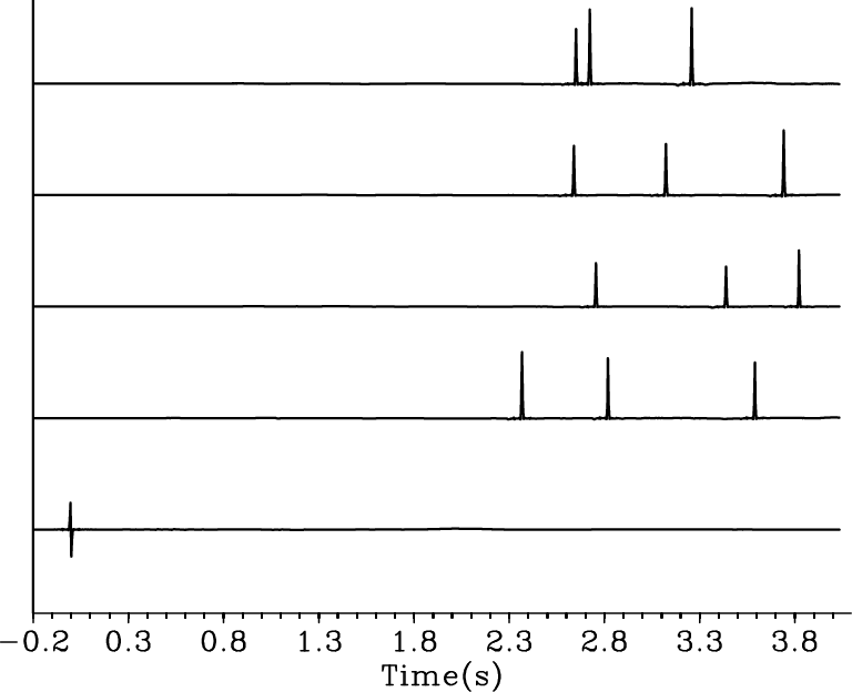
Claerbout et al. (2012) provide the complete, step-by-step derivation of the gain function in the Fourier-domain bidirectional deconvolution approach. I test the this gain method on a simple synthetic data example. I use a five-trace simple spiky reflectivity model convolved with a zero-phase synthetic wavelet to make the synthetic data. In particular, I put a dipole at the beginning of the fifth trace of the model. If the deconvolution honors the beginning more than the end of the traces, it will tend to make one spike rather then a dipole at that location in the output. On the other hand, if the deconvolution does not incorrectly emphasize the beginning of the traces, we will get a dipole back. Figure 4 shows the synthetic model and wavelet, and Figure 5 shows the synthetic data without and with decay. Figure 6 shows the recovered wavelet and model by deconvolution without gain. Because there is no decay in the data, the result is nearly perfect. Then I add a decay to the model, proportional to the time squared. Figure 7 shows the recovered wavelet and model by deconvolution of this decaying data without gain. So that the decayed end of the traces would be evident, I applied a time-squared scale on the time axis in Figure 7(b). The results are poor; there is only a spike rather than a dipole at the beginning of the fifth trace in the output. However, when I include the gain function in the deconvolution following the implementation discussed above, I get the results shown in figure 8. I also applied a time-squared scale on the time axis in Figure 7(b). By including the gain function in the deconvolution to correctly balance the amplitudes, I can get nearly perfect results again.

fig-8a,fig-8b
Figure 4. Wavelet (a) and five-trace model (b) used for synthetic example.

fig-85a,fig-85b
Figure 5. Five-trace synthetic data set without (a) and with decay proportional to the time squared (b).

fig-9a,fig-9b
Figure 6. Estimated wavelet (a) and recovered result (b).

fig-10a,fig-10b
Figure 7. Estimated wavelet (a) and recovered result (b) of decay data without gain. For easily see the decayed end of the traces, a time squared scale are applied on the time axis in the result (b).

fig-11a,fig-11b
Figure 8. Estimated wavelet (a) and recovered result (b) of decay data with gain. For easily see the decayed end of the traces, a time squared scale are applied on the time axis in the result (b).

Recent progress regarding logarithmic Fourier-domain bidirectional deconvolution