P/S separation of OBS data by inversion in a homogeneous medium

Synthetic land data 2

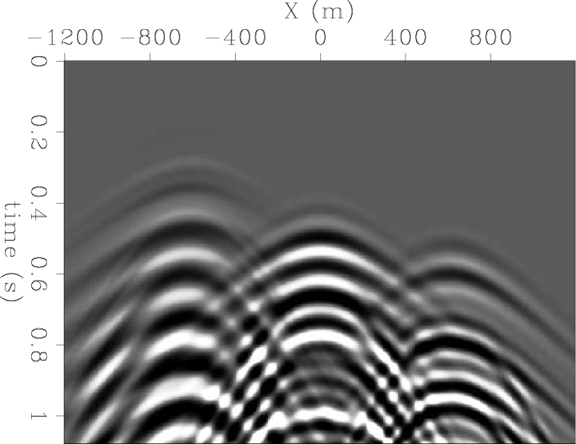
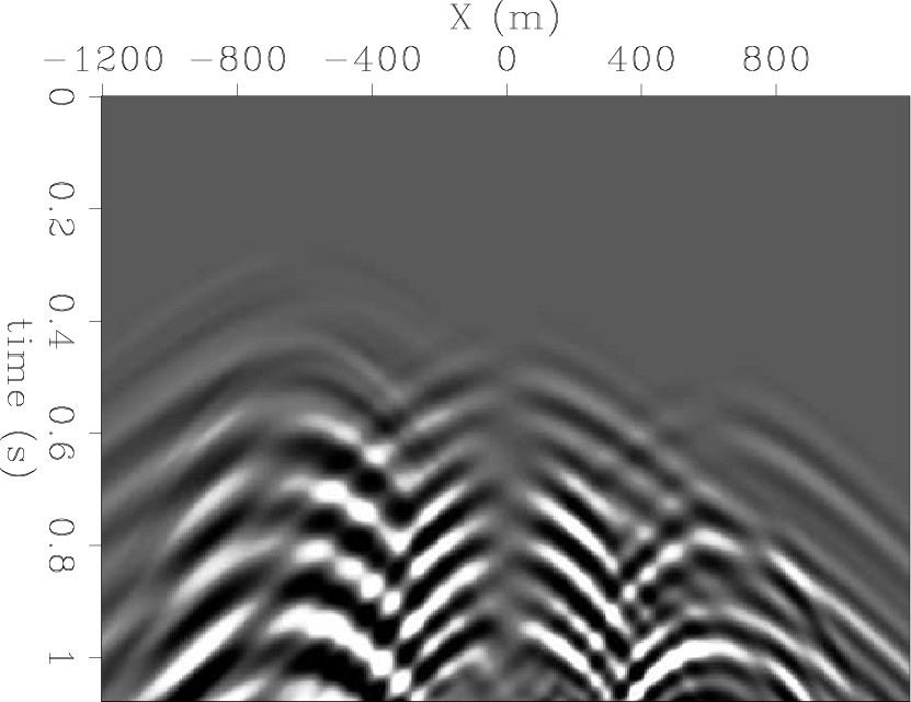
The next set of examples are also of synthetic land data, but they represent a scenario where the velocity at the recording surface varies laterally. Three shot gathers were generated in three separate homogeneous mediums, with differing medium parameters. For each gather there was a different random reflection series. The gathers were then summed to simulate a variable surface velocity.

The forward modeling medium parameters were:

1. Gather 1: $v_{p1} = 2000 \frac{\text m}{\text s}, \quad \quad v_{s1} = 1000 \frac{\text m}{\text s}, \quad \quad \rho_1 = 2.0 \frac{gr}{cm^3}$
2. Gather 2: $v_{p2} = 1800 \frac{\text m}{\text s}, \quad \quad v_{s2} = 900 \frac{\text m}{\text s}, \quad \quad \rho_2 = 1.8 \frac{gr}{cm^3}$
3. Gather 3: $v_{p3} = 1600 \frac{\text m}{\text s}, \quad \quad v_{s3} = 800 \frac{\text m}{\text s}, \quad \quad \rho_3 = 1.6 \frac{gr}{cm^3}$

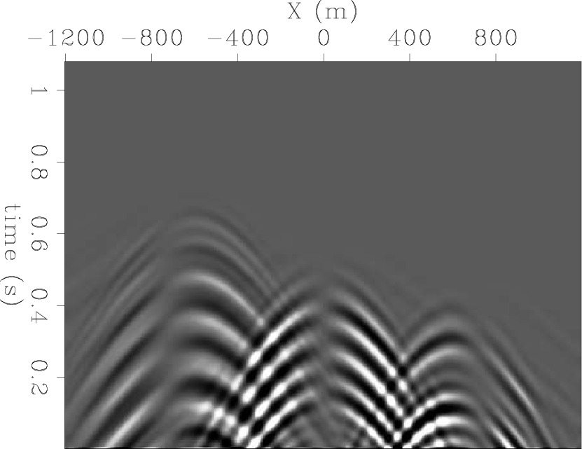
Figures 9(a) and 9(b) are the vertical and horizontal displacements. Figures 9(c) and 9(d) are the P and S-waves calculated by applying the Helmholtz separation operators. Three different reflection groups can be discerned in the synthetic data. The left group corresponds to the fastest medium, the central group to the intermediate medium, and the right group to the slowest medium.

lu2-0,lu2-1,lp2-0L,lp2-1L
Figure 9. Synthetic land data. (a) vertical displacement, (b) horizontal displacement, (c) P-wave, (d) S-wave.

There were three inversion runs, each one with different homogeneous medium parameter sets:

1. Inversion 1 (intermediate): $v_{p1} = 1700 \frac{\text m}{\text s}, \quad \quad v_{s1} = 850 \frac{\text m}{\text s}, \quad \quad \rho_1 = 1.7 \frac{gr}{cm^3}$
2. Inversion 2 (slow): $v_{p2} = 1500 \frac{\text m}{\text s}, \quad \quad v_{s2} = 700 \frac{\text m}{\text s}, \quad \quad \rho_2 = 1.5 \frac{gr}{cm^3}$
3. Inversion 3 (fast): $v_{p3} = 2000 \frac{\text m}{\text s}, \quad \quad v_{s3} = 1000 \frac{\text m}{\text s}, \quad \quad \rho_3 = 2.0 \frac{gr}{cm^3}$

The medium parameters of inversion $3$ match those of the fast events, but are different from the parameters used to generate the intermediate and the slow events. As for the medium parameters of inversions $1$ and $2$ , they match none of the parameters used to generate the datasets. For inversion $2$ , the velocity error is up to $33\%$ (compared to the fast arrivals). The inversions were run until a good match to the displacement data was achieved.

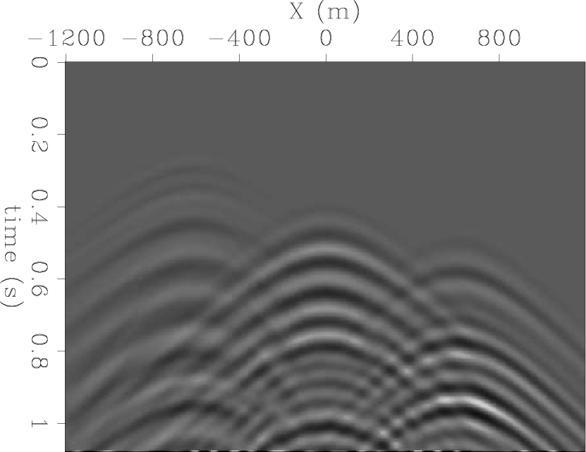
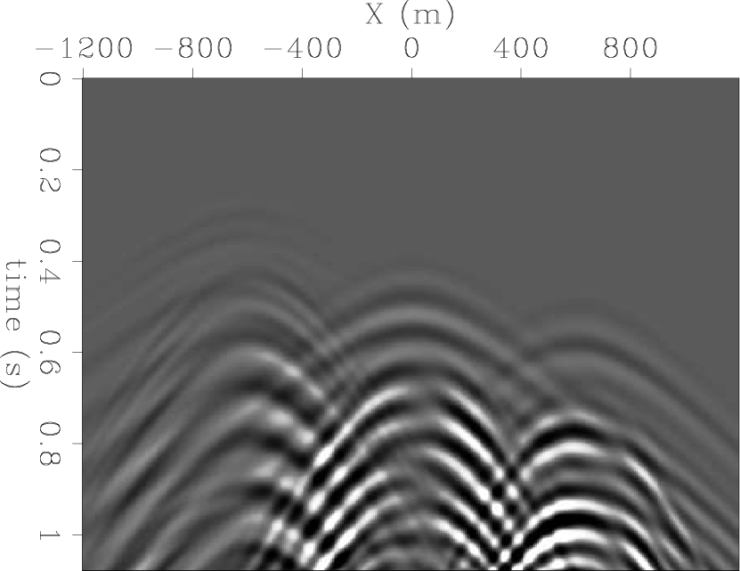
Figures 10(a)-10(e) show the reconstructed P-waves. Figure 10(a) is the synthetic P recording. Figure 10(b) is the P reconstruction calculated from the displacements of the inversion with parameter set $1$ (intermediate). Figure 10(c) is the P reconstruction from the inversion using parameter set $2$ (slow), and Figure 10(d) is from parameter set $3$ (fast). Figure 10(e) is the summation of the synthetic P and S recordings, and is a visual aid to estimate the separation quality for each scenario.

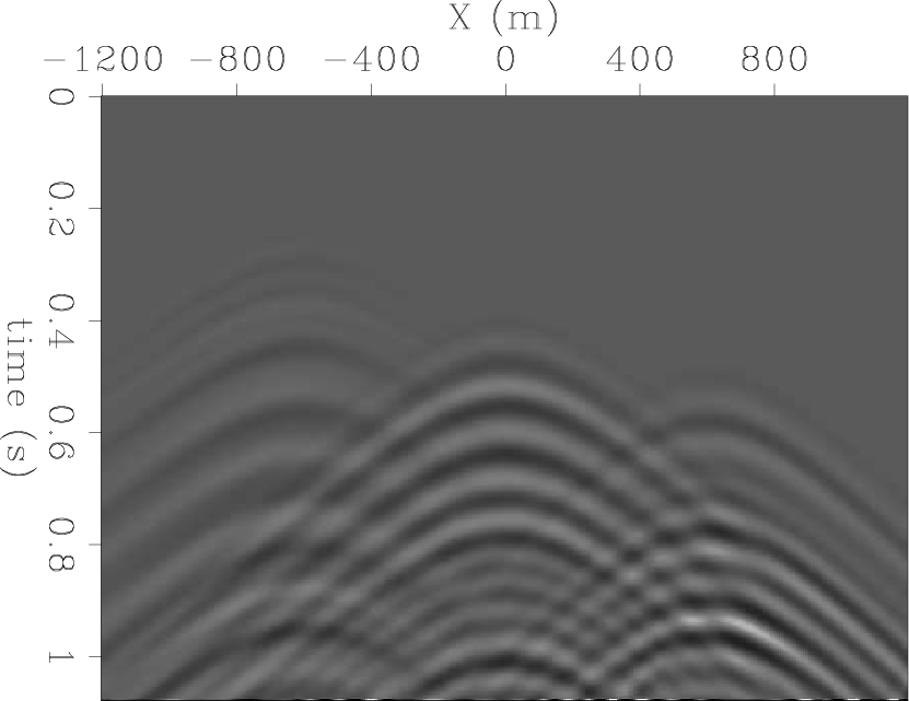
Since the intermediate parameter set $1$ has the least error in comparison to the media with which the forward modeled data were generated, the reconstructed P-wave is most accurate for it, as seen in Figure 10(b). However, the other two P-wave reconstructions show reasonable separation quality, despite the large error in medium parameters. The same can be said for the next set of S-wave separation results in Figures 11(a)-11(e). The best separation is where the medium parameter error is minimal (Figure 11(b)). However, even where the error is large (Figures 11(c) and 11(d)), the separation results, though not being great, are still reasonably good compared to the synthetic data.

lp2-0,lp2-2,lp2-4,lp2-6,lp2-8L
Figure 10. Synthetic and reconstructed P-wave of land data. (a) Synthetic P, (b) reconstructed P with intermediate medium parameters, (c) reconstructed P with slow parameters, (d) reconstructed P with fast parameters, (e) sum of synthetic P and S-waves. All figures are identically clipped.

lp2-1,lp2-3,lp2-5,lp2-7,lp2-8
Figure 11. Synthetic and reconstructed S-wave of land data. (a) Synthetic S, (b) reconstructed S with intermediate medium parameters, (c) reconstructed S with slow parameters, (d) reconstructed S with fast parameters, (e) sum of synthetic P and S-waves. All figures are identically clipped.

P/S separation of OBS data by inversion in a homogeneous medium