|
|
|
|
Wave-equation migration velocity analysis for anisotropic models on 2-D ExxonMobil field data |
 .
.
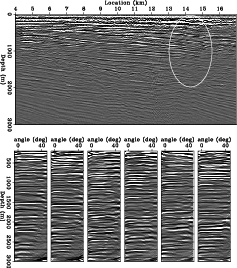
We can see many small-scale faults in this area on the top panel in Figure 6. Migration artifacts at  km
and
km
and  m are caused by a big vertical fault running from
  km on the top to the bottom of the section.
The initial angle gathers are shown in the bottom row in Figure 6. Since this is a streamer geometry, the subsurface reflectors are only
illuminated from positive angles. Although the gathers are almost flat, we can still see upward
residual moveouts in the angle domain. Therefore, we have a chance to improve the model and the image by flattening the gathers.
km on the top to the bottom of the section.
The initial angle gathers are shown in the bottom row in Figure 6. Since this is a streamer geometry, the subsurface reflectors are only
illuminated from positive angles. Although the gathers are almost flat, we can still see upward
residual moveouts in the angle domain. Therefore, we have a chance to improve the model and the image by flattening the gathers.
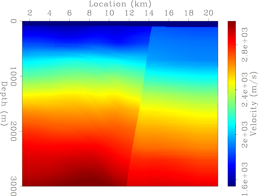
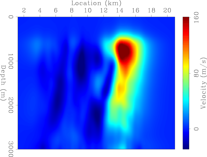
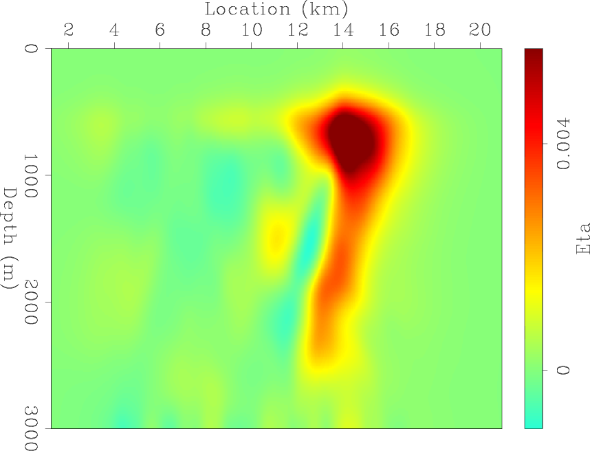
Updates between the initial and the inverted velocity and
models are shown in Figure 5(a) and Figure 5(b),
respectively. First, notice the spatial correlation between velocity updates and
updates, although no such constraints are applied during the inversion.
However collocated, the update directions in velocity and
are not necessarily the same. We are able to resolve a localized shallow anomaly between  km
and
km
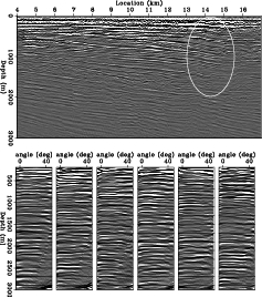
and  km at around 800 m below surface. Comparing the initial stack image on the top panel in Figure 6 with the final stack image on the top
panel of Figure 7, we can see improved continuity and signal strength in the area highlighted by the oval. The fault in this area is also better defined
in the final image. Notice that the updates in velocity are less than 10%, whereas the updates
in
are around 25%. These positive updates in both velocity and
agree well with the negative travel time misfits in the previous OCS modeling results
(Figure 1).
km at around 800 m below surface. Comparing the initial stack image on the top panel in Figure 6 with the final stack image on the top
panel of Figure 7, we can see improved continuity and signal strength in the area highlighted by the oval. The fault in this area is also better defined
in the final image. Notice that the updates in velocity are less than 10%, whereas the updates
in
are around 25%. These positive updates in both velocity and
agree well with the negative travel time misfits in the previous OCS modeling results
(Figure 1).
We can also verify the updates in velocity and
on the angle gathers at different CMP locations. The initial angle domain common image gathers (ADCIGs) are shown in the
bottom row in Figure 6, and the final ADCIGs produced using the inverted models are shown in the bottom row in Figure 7.
To better illustrate the effects of the model updates, the ADCIGs are sampled more densely between CMP =
and  and sparsely outside of this range.
In general, we can see improved flatness for all the reflectors. Specifically, for the shallower events above
and sparsely outside of this range.
In general, we can see improved flatness for all the reflectors. Specifically, for the shallower events above  km, most improvements happen at large angles over
 . Therefore, we interpret the improvements for the shallow events primarily as the contribution of the improved
model.
. Therefore, we interpret the improvements for the shallow events primarily as the contribution of the improved
model.
For the deeper events at the same CMP location, both the depth and the flatness of the angle
gather have been changed by inversion. The upward-curving events in the angle domain from the initial migration has been flattened by the improved velocity and
model. This result would be more convincing if we had the corresponding well logs at the same location to verify the depth shifts.
|
|---|
|
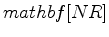
dip-exxon
Figure 3. Estimated dip field from the initial image on the top panel of Figure 6. |
|
|
|
|---|
|
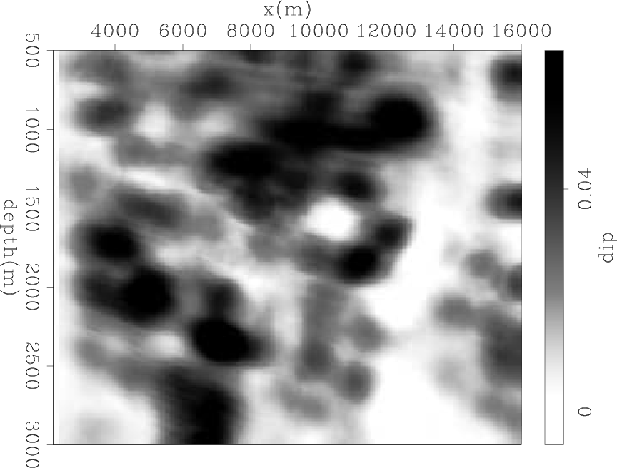
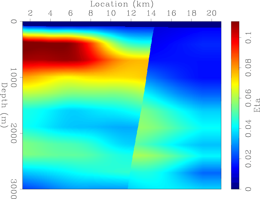
initv,inite
Figure 4. Initial velocity model (a) and initial
model (b).
|
|
|
|
|---|
|
vchange,echange
Figure 5. Updates in velocity model (a) and updates in
model (b) after inversion.
|
|
|
|
|---|
|
image-init-an
Figure 6. The initial stack image (Top panel) and initial angle domain common image gathers at CMP  km (Bottom row).
|
|
|
|
|---|
|
image-fnal-an
Figure 7. The final stack image (Top panel) and final angle domain common image gathers at CMP
km (Bottom row). Compared
with Figure 6, improvements in continuity and enhancements in amplitude strength are highlighted by the oval.
|
|
|
|
|
|
|
Wave-equation migration velocity analysis for anisotropic models on 2-D ExxonMobil field data |