|
|
|
|
Wave-equation migration velocity analysis for anisotropic models on 2-D ExxonMobil field data |
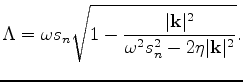
We parameterize the VTI subsurface using NMO slowness  , and Thomson parameters
  and
and
 (Thomsen, 1986).
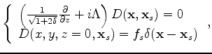
In the shot-profile domain, both source wavefields
(Thomsen, 1986).
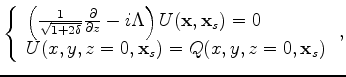
In the shot-profile domain, both source wavefields  and receiver wavefields
  are
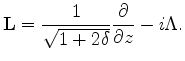
downward continued using the following one-way wave equation and boundary condition
(Shan, 2009):
are
downward continued using the following one-way wave equation and boundary condition
(Shan, 2009):
Equations 1 and 2 can be summarized in matrix forms as follows:
 |
(6) |
 |
(7) |
 |
(8) |
It is well known that parameter
is the least constrained by surface seismic data
because of
the lack of depth information. Therefore, we assume
can be correctly obtained from other
sources of information, such as check shots and well logs. In this paper, we are going to invert for
NMO slowness
and
.
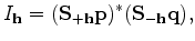
We use an extended imaging condition (Sava and Formel, 2006) to compute the image cube with subsurface offsets:
 is a shifting operator which shifts the wavefield
 in the
  direction. Notice that
 .
Equations 4, 5 and 9 are state equations, and
,
and
.
Equations 4, 5 and 9 are state equations, and
,
and  are the state variables.
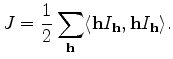
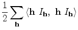
To evaluate the accuracy of the subsurface model, we use a DSO objective function (Shen, 2004):
 is the subsurface offset. In practice, other objective functions (linear transformations of the image) can be used rather than DSO. To derive the DSO objective function with respect to
and
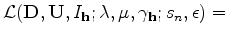
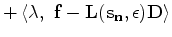
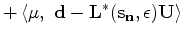
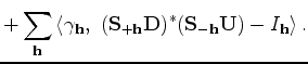
, we follow the recipe provided by Plessix (2006). First, we form the Lagrangian augmented functional:
is the subsurface offset. In practice, other objective functions (linear transformations of the image) can be used rather than DSO. To derive the DSO objective function with respect to
and
, we follow the recipe provided by Plessix (2006). First, we form the Lagrangian augmented functional:
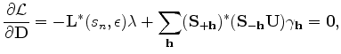
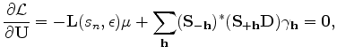
Then the adjoint-state equations are obtained by taking the derivative of
 with respect to state variables
,
and
:
with respect to state variables
,
and
:
 ,
,  and
and
 are the adjoint-state variables, and can be calculated from the
adjoint-state equations.
are the adjoint-state variables, and can be calculated from the
adjoint-state equations.
The physical interpretation of the adjoint-state equations offers better understanding of the physical
process and provides insights for implementation. Clearly, the solution to equation 15,
, is the perturbed (residual) image at a certain subsurface offset. Equations 13
and 14 define the perturbed source and receiver wavefields, respectively. Notice the perturbed
source wavefield
at location
depends on the image at
 and the background receiver wavefield
at
and the background receiver wavefield
at
 .
The same rule applies to the perturbed receiver wavefield
.
.
The same rule applies to the perturbed receiver wavefield
.
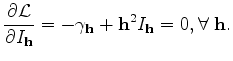
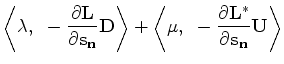
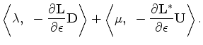
With the solutions to the equations above, we can now derive the gradients of the objective function
10 by taking the derivative of the augmented functional
with respect to the
model variables
and  as follows:
|
|
|
|
Wave-equation migration velocity analysis for anisotropic models on 2-D ExxonMobil field data |