|
|
|
|
VTI migration velocity analysis using RTM |
 :
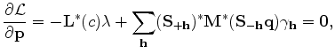
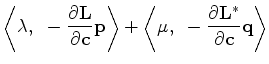
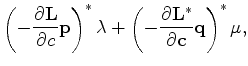
with respect to state variables
:
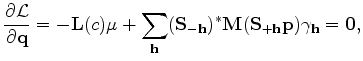
with respect to state variables  ,
,  and
and  :
:
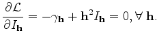
 and
and
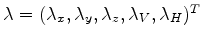
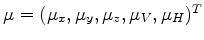 are the adjoint-state fields and the
solution of the adjoint-state equations 25 and 26. Variable
are the adjoint-state fields and the
solution of the adjoint-state equations 25 and 26. Variable
 is the scaled image slice at the subsurface offset
  .
.
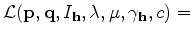
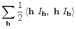
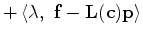
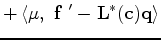
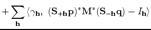
Now the gradient of the objective function 15 with respect to velocity is:
|
|
|
|
VTI migration velocity analysis using RTM |