How incoherent can we be? Phase-encoded linearised inversion with random boundaries

Inversion With Random Boundaries

Under a single Born scattering assumption we can describe the recorded data as

$$d(\mathbf x_r, \mathbf x_s,\omega)=\sum\limits_{\mathbf x_s,\omeg... ...mega)m(\mathbf {x})\sum\limits_{\mathbf x_r}G_0(\mathbf x, \mathbf x_r,\omega).$$ (1)

The adjoint process can thus be written as

$$m(\mathbf {x})=\sum\limits_{\mathbf x_s,\omega}f(\omega) G_0(\mat... ...hbf x_r}G_0(\mathbf x, \mathbf x_r,\omega)d^*(\mathbf x_r, \mathbf x_s,\omega).$$ (2)

Where $d$ is the data, $G_0$ are the respective Green's functions, $m$ the model, $\mathbf {x}$ the three-dimensional model coordinate, $\mathbf x_{r,s}$ the three-dimensional source and receiver coordinates, $\omega$ temporal frequency, $f(\omega)$ the source waveform and $*$ denotes the complex conjugate. It is this complex conjugate that reverses the sense of time, meaning that in the time domain we back propagate the source and receiver wavefields and correlate them at each imaging time step. This complex conjugate and the subsequent source wavefield modelling create the need for either saving this wavefield or forming a time-reversible source wavefield. Random boundaries scatter this wavefield incoherently whilst adhering to the conservation of energy; after propagation correlation and stacking will reduce residual noise.

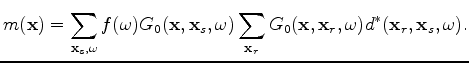
Random boundary noise in an RTM image is stacked out at a rate of $\sqrt N$ , where N is the number of sources; often we see better performance than this. By using a different random boundary for each shot experiment we see random noise levels at an acceptable level after combining around 50 shots. Some effects of this can be seen below, where we use a GPU based RTM algorithm and model and migrate 100 shots over a section of the SEAM velocity model (Figure 1), simulating a marine survey. We then perform 5 iterations of least-squares linearised inversion with the same dataset. Here we have 50 inline shots at 100m spacing, 2 crossline shots with 1km spacing and 825x200 receivers. Comparison of such a scheme compared to source saving are shown in Clapp (2009).

srfl2 Figure 1. A 2D slice from the reflectivity model that we are attempting to recover.

imgc2
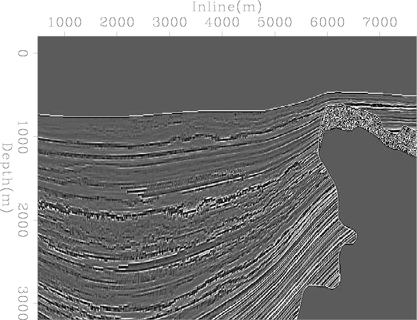
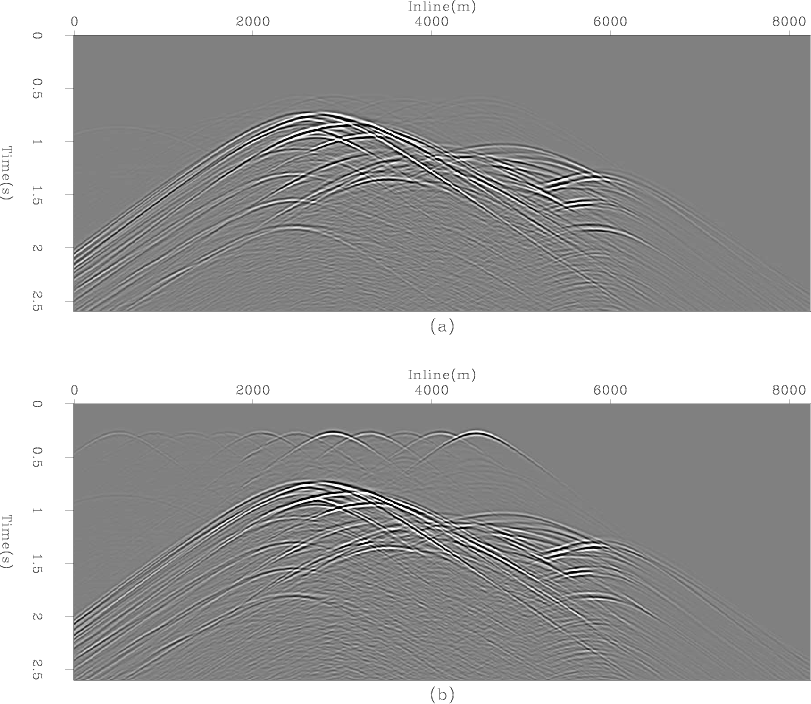
Figure 2. RTM and linearised inversion example 2D slices. (a) shows the raw RTM result, (b) raw inversion after 5 iterations, (c) is (a) after a lowcut wavenumber filter and (d) is (b) after the same lowcut filter.

As expected, in Figure 2 we see image quality improve when extending this procedure to an iterative least squares inversion. The footprint from the limited acquisition begins to dissipate and we see generally higher frequency content and more balanced, geologically accurate amplitudes. However, since only a limited number of iterations have been performed some artefacts remain, from both the random boundaries and from the inverse system.

datac
Figure 3. An example of source self-correlation. a) shows the real data after encoding 10 shots. b) shows the modelled data when the water column noise has not been muted. Artifacts similar to direct arrivals not present in a) can be seen.

When blindly extending this process to an inversion, relatively poor convergence can be seen, especially with respect to the data space residual. The reason for this can be seen when looking at this residual. The random boundary image (the gradient, in this case) features noise in the water column and a source location imprint artefact. When modelling data over this image we see an artefact manifested as a direct arrival from the source self-correlating. This can be removed by either muting the water column in the image or by time muting the remodelled data before back-propagation. An example of this under a phase-encoded setting is shown in Figure 3. Furthermore, we can improve convergence by changing the random boundaries as a function of iteration number, as well as a function of shot position.

The computational advantage for GPU based RTM is considerable. We can consider three scenarios - when the source wavefield must be entirely saved to disk, when the source wavefield can held in the CPU memory and when using random boundaries. One should note the last of these requires an extra computation - the source wavefield back propagation during RTM. In total computation time asynchrous disk wavefield transfer is nine times slower than random boundary RTM, and if the source wavefield can be compressed and stored on the CPU memory this is 1.5 times slower. Of course, these conclusions are strongly related to the speed of the disks being used.

timec
Figure 4. Compute time comparisons for three RTM regimes. Green denotes IO, yellow propagation, blue damping, red injection and purple imaging. (a) uses asynchronous disk transfers, (b) assumes the entire source wavefield can be held in CPU memory and (c) uses random boundaries.

How incoherent can we be? Phase-encoded linearised inversion with random boundaries