How incoherent can we be? Phase-encoded linearised inversion with random boundaries

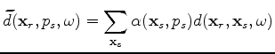
Phase Encoding With Random Boundaries

Phase encoding can have multiple meanings; herein we describe the process of weighting and combining shots to reduce data size. We do this by creating a matrix of weights and applying it to our data.

$$\widetilde{d}(\mathbf x_r,p_s,\omega) = \sum\limits_{\mathbf x_s} \alpha(\mathbf x_s,p_s)d(\mathbf x_r,\mathbf x_s,\omega)$$ (3)

Now $\widetilde{d}$ denotes our phase encoded data, $\alpha$ is a sequence randomly selecting either 1 and -1, and $p_s$ is some sort of realisation index. When combining all shots together $p_s$ will be 1. For the forward process we propagate a source function encoded with the same sequence $\alpha$ .

Augmenting random boundary linearised inversion with phase encoding requires some additional thought. In the case where we combine all shots to one super shot, we are now propagating 100 weighted shots through the same random boundary. On a shot by shot basis this is acceptable, as each wavefield will be incident on the boundary at a different angle and hence scatter differently. However, when performing this conventionally we formulate a gradient for each shot separately and then sum them to create our final gradient, reducing our noise by $\sqrt N$ . Furthermore, there are only two coherent wavefields (the source and receiver) that can correlate with the scattered field to induce noise. When combining all shots together, we do not quite see this behaviour because we now have every scattered field (unique per shot) correlating with every scattered field and with every coherent field, of which there are now $2N$ . Fortunately, the correlation of scattered fields should also be a random walk reduction at $\sqrt N$ . Typically with phase encoded linearised inversion after $nshots$ iterations one expects to see an acceptably clean image. When including random boundaries we see a noisier image, as expected, but all key features are present. Images can still be artefact-laden, especially in areas of low illumination, but this is typical of both random boundary and phase-encoded imaging when done independently.

We have several options to mitigate this. The best results are seen by combining several random subsets of shots, calculating a gradient for each subset and combining these to form the gradient for a single iteration. Whilst this appears more computationally demanding, the fact that single super-shot GPU based inversion is not further parallelisable over shots makes this approach seem more appealing. Over a node containing 8 Fermi M2090 cards we can create the gradient for 8 different super shots and combine these for little extra time cost, giving a cleaner gradient per iteration. We now see more favourable convergence characteristics and slightly cleaner images. With naive phase encoded inversion we see a convergence to 60% within the data-space residual norm after 100 iterations with 50 combined shots. With a water column mute applied we see convergence to 56% and with multiple, stacked realisations we see convergence to 53%. Once the data error is below 50% we tend to see very gradual improvements for all situations. One full, non-encoded iteration with random boundaries (roughly the same cost) takes us to 74% data error.

sicr Figure 5. The reflectivity model that we are inverting for.

sic
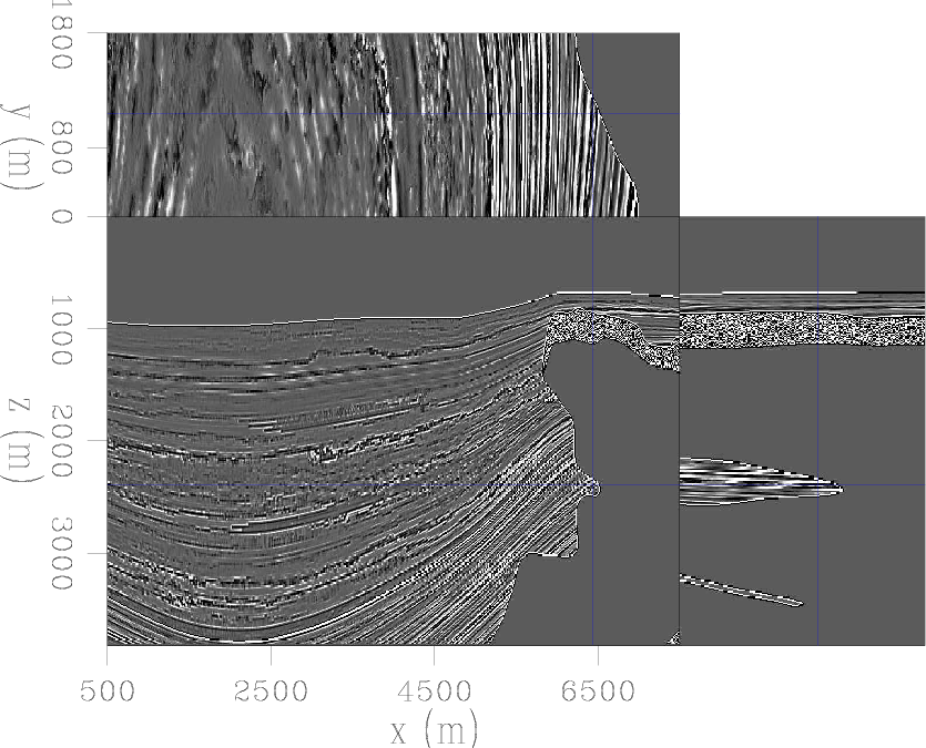
Figure 6. Linearised inversion examples. (a) shows the model after one iteration of conventional inversion, (b) the model after two iterations, (c) phase encoded inversion after 80 iterations - equivalent cost to (a) and (d) phase encoded inversion after 160 iterations - equivalent cost to (b).

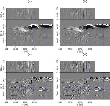
Figure 6 compares the results of conventional, separated linearised inversion with phase encoded inversion, over the 3D model shown in Figure 5. Here we had 120 shots in total, 60 inline at 100m spacing and two crossline at 1km spacing. Again, receivers were in a 825x200 grid. Images (a) and (c) are equivalent in computational cost, as are images (b) and (d). The first noticeable aspect are the low-frequency artefacts present in the non-encoded image. These occur due to wavefields moving in the same direction correlating and are prevalent over high-reflectivity, high-contrast features such as salt boundaries. Often the first several iterations of linearised inversion will work on removing these artefacts before focusing on other areas, as can also be seen in Figure 2. The second noticeable aspect is that the frequency content of the phase encoded image is much higher. The resolution, especially on the salt edges, is greater; high-frequency noise is also present, but this is expected. The additional iterations performed here have successfully begun to remove the effect of the source wavelet in the image, whereas in the RTM image this wavelet is squared. Figure 7 shows these same images after a low-cut bandpass filter and some light amplitude gain. The filter has removed the low-wavenumber noise, but at the expense of the vertical salt edge. The conventional images look much improved, but the resolution and general content of the phase-encoded images still seem preferable.

sicc
Figure 7. The same set of results as in Figure 6 but each with a low-cut spatial frequency filter and some amplitude gain.

Figures 6 and 7 show that for equivalent cost, even when augmented with random boundaries, phase encoded linearised inversion can yield high quality images. This scheme is also incredibly well-adapted for GPU computing - there is no IO during propagation in the forward or adjoint scheme, and the objects we need to copy to the GPU are all the size of the model, the size of one shot, or smaller.

peres
Figure 8. Normalised residual evolution as a function of iteration number.

Residual behaviour with iteration number can be seen in Figure 8. As a reference point for separated inversion after two iterations the respective normalised residual difference norms (normalised to 100) were 88.9 and 79.9, which are not significantly smaller than those shown. However, in terms of cost the former of these would appear at 80 iterations, the latter at 160. With this is mind we see that our phase-encoding scheme is doing a vastly more efficient job at data fitting, in an $l_2$ sense. However, when interpreting these scalar fits we must consider that the $l_2$ residual norm does not well represent high-frequency noise, and so two images with an apparently similar residual may have quite different high-frequency noise characteristics. It is due to this that we must take the phase encoded scheme to so many iterations. Typically, we will need at least $nshots/2$ if not $nshots$ iterations for a clean image here. With conventional inversion we need 5-10 iterations to remove the low-frequency salt artefacts and many more for amplitude and acquisition imbalances.

How incoherent can we be? Phase-encoded linearised inversion with random boundaries