Data examples of logarithm Fourier-domain bidirectional deconvolution

Field data common-offset gather example

Now we test the logarithm Fourier-domain bidirectional deconvolution with a 2D marine common offset gather data set that is commonly used to test the time-domain bidirectional deconvolution methods. This 2D marine common-offset gather is very popular in papers discussing blind deconvolution using the hyperbolic penalty function. In Zhang and Claerbout (2010a), Zhang and Claerbout (2010b), Fu et al. (2011), Shen et al. (2011a) and Shen et al. (2011b) the authors tested their methods and theories with this data set as a field data example. Hence this is a good choice for comparing this new method with previous ones.

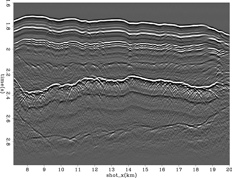
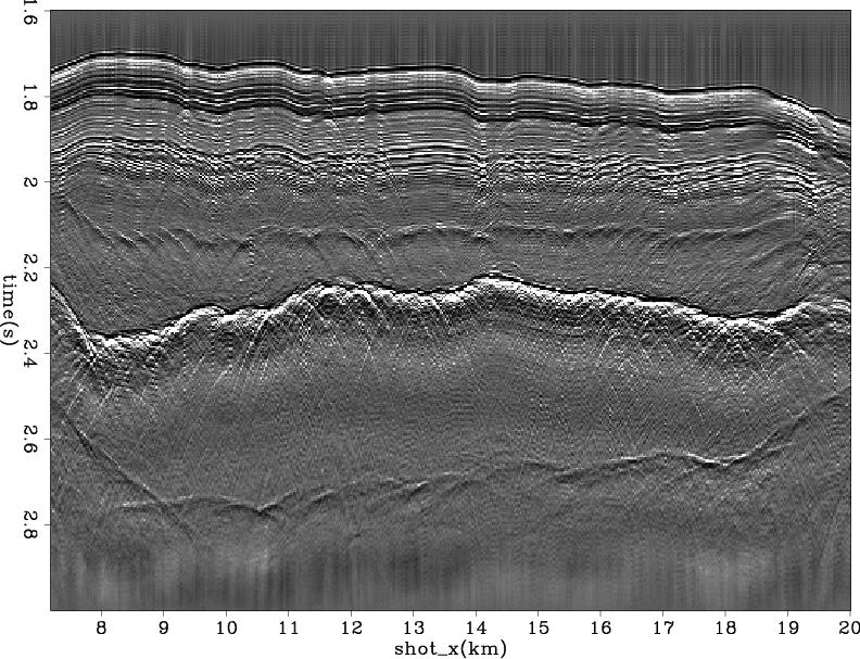
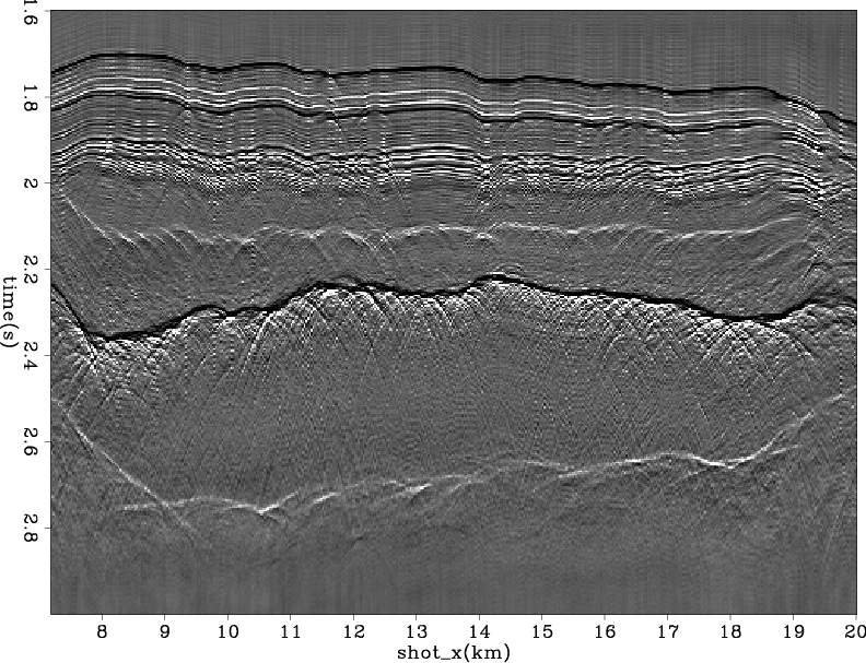
Figure 2 shows the 2D marine common offset gather. Figure 3 shows the common-offset section after Burg PEF preconditioning. Figures 4 and 5 compare the results of two methods of bidirectional deconvolution.

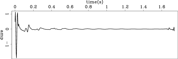
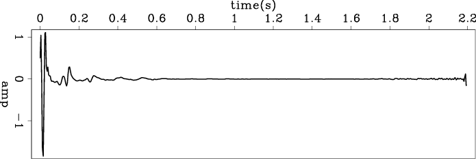
Figures 6(a) and 6(b) show the comparison of the estimated wavelets from the two methods. Recall that the estimated wavelet is the inverse deconvolution filter. We get the inverse filter by inverting the frequency spectrum of the filter in the Fourier domain, so the wavelet waveform is periodic. This means the jitter we see at the end of the wavelet is the anti-causal part of the filter.

From figures 4 and 5, both methods provide good quality results. However we think the logarithm Fourier-domain method (figure 4) is a little better. First, there are fewer precursors in the the logarithm Fourier domain result than in the time domain result. And the precursor of the logarithm Fourier-domain result does not have a sharp boundary as the precursor of the time domain result. The sharp boundary of the time domain result is caused by the anti-causal deconvolution filter $b$ , which is 20 sample long, and a sharp boundary on the beginning of the anti-causal deconvolution filter $b$ . Because the logarithm Fourier-domain uses a periodic deconvolution filter, the anti-causal part of the deconvolution filter has no beginning. Moreover, within the salt body (in the vicinity of 2.4 s to 2.6 s), the Fourier-domain result looks cleaner. We find within the salt body, there are fewer low frequency events (which can be seen as the white stripe in figure 5 within 2.4 s to 2.6 s). We do not expect to see any features within the salt body, therefore all events we see in this area in the raw data are the air-gun bubbles. This indicates that the Fourier-domain deconvolution handles the air-gun bubbles better than the time-domain method. However, excluding these differences, the results are similar. We can also find that, except for the tail parts, the estimated wavelets (figures 6(a) and 6(b)) are similar. At the tail of the wavelet which, because of periodicity, correspond to the anticausal part of the logarithm Fourier domain wavelet the wavelet estimated by the time domain symmetric method has less jitter. On the contrary, the logarithm Fourier-domain wavelet appears to have a small anti-causal air-gun bubble.

Here, we have a paradox. From the comparison of deconvolution result (figures 4 and 5), we conclude that in terms of quality, the the logarithm Fourier-domain method is better. But from the wavelet comparison, we can reach an oppsite conclusion. This is because the deconvolution filter in the logarithm Fourier-domain method is periodic and the length of anti-causal part has not an extra constraint, whereas the anti-causal filter in the time domain symmetric method is constrained by the anti-causal filter length parameter and tends to have less anti-causal jitter in the final estimated wavelet.

cof-data
Figure 2. A common-offset section of a marine survey.

cof-data-decon
Figure 3. The common-offset section after applying the Burg PEF preconditioner.

cof-data-log
Figure 4. Logarithm Fourier-domain bidirectional deconvolution result.

cof-data-linear
Figure 5. Time-domain (symmetric) bidirectional deconvolution result.

wavelet-cof-data-linear,wavelet-cof-data-log
Figure 6. Estimated wavelet from (a) logarithm Fourier-domain and (b) time-domain (symmetric) bidirectional deconvolution. The estimation wavelets are the inverse deconvolution filters, calculated by inverting the frequency spectrum of the filter in the Fourier domain. Therefore the wavelet waveform is periodic, and the jitter we find at the end of the wavelet is the anti-causal part of the filter.

Data examples of logarithm Fourier-domain bidirectional deconvolution