Data examples of logarithm Fourier-domain bidirectional deconvolution

Synthetic 1D example

First, we demonstrate the advantage of the logarithm Fourier-domain method over the time-domain method on a very simple synthetic data example. The input is a Ricker wavelet generated by an approximate approach that applies a second-order derivative to binomial coefficients (Fu et al., 2011). Figure 1(a) shows a synthetic Ricker wavelet, and 1(b) shows the Ricker wavelet after Burg PEF preconditioning. Next we use the symmetric method (Shen et al., 2011a) to perform time-domain bidirectional deconvolution. Figures 1(c) and 1(d) compare the results of bidirectional deconvolution using the two methods.

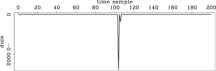
For this simple 1D synthetic example, we use 0.1 (which is 5% of the peak amplitute of the input) as the threshold of the hyperbolic penalty function for the logarithm Fourier-domain method and use 95% quantile of the data residual as the threshold for the time-domain method. Using the logarithm Fourier-domain method, we turn the Ricker wavelet into a spike output after about 50 iterations. Using the time-domain symmetric method, even after 30,000 iterations, we get a major spike followed by a minor spike, plus a few additional jitters at the begining of the trace. At the time of this publication, we do not fully understand why the symmetric method, which utilizes a conjugate direction solver, is significantly slower than the logarithmic method, which utilizes a steepest descent algorithm.One possible explanation, which has not been tested, is that the deconvolution filters derived from the time domain symmetric method are not strictly minimum and maximum phase wavelets.

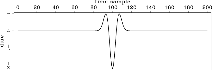
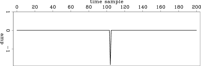
Another important observation from this synthetic test case is the output location of the bidirectional deconvolution. If we check the wiggles carefully, we can measure that the major peaks of the two deconvolution results in figures 1(c) and 1(d) (both of which are at time sample 104) are not the same as the location of the major peak of the input data figure 1(a) (which is at the time sample 100). Instead, they are located at the major peak location of the preconditioning result in figure 1(b). This inspired us to realize that the output spike location of the deconvolution is determined by the preconditioner, and that we can change the preconditioner to move the spike of the deconvolution result to the location desired. In another paper (Shen et al., 2011b), we discuss this interesting topic in more detail.

ricker,ricker-decon,ricker-log,ricker-linear
Figure 1. (a) The synthetic Ricker wavelet; (b) The Ricker wavelet after Burg PEF preconditioning; (c) The bidirectional deconvolution result of the logarithm Fourier-domain method after 50 iterations; (d) The bidirectional deconvolution result of the time-domain symmetric method after 30,000 iterations.

Data examples of logarithm Fourier-domain bidirectional deconvolution