Subsalt imaging by target-oriented wavefield least-squares migration: A 3-D field-data example

Inversion result

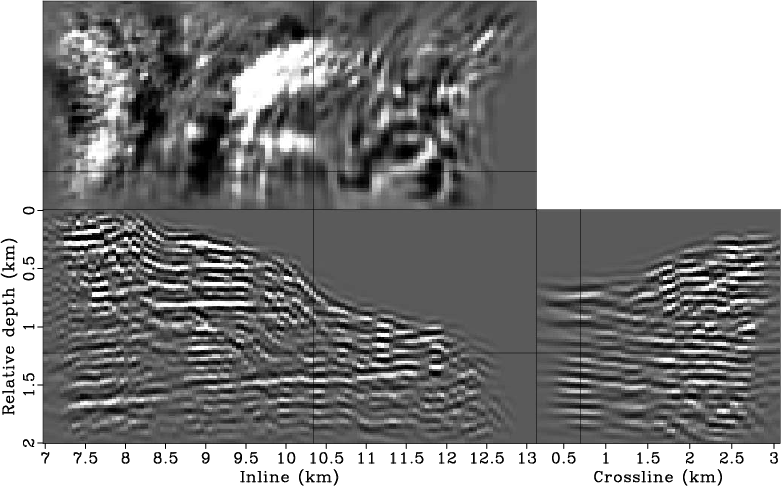
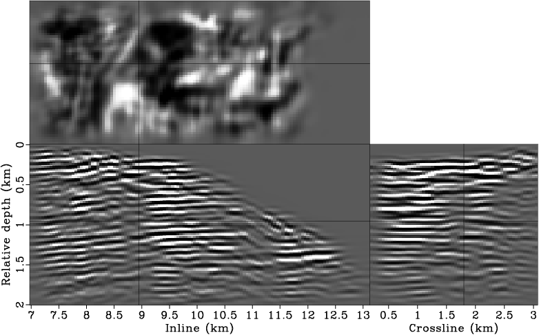
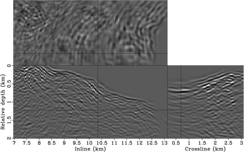
Since the goal is to invert sediment reflectivities, we incorporate a mask operator (Figure 7) into the inversion to prevent updating the reflectivities of the salt boundary. We first run the inversion without applying any regularizations; the inverted image after $100$ iterations is shown in Figure 9. Compared to migration (Figure 8), inversion significantly improves the spatial resolution of the image; the amplitudes are more balanced, and the illumination shadows are filled in. However, the inverted image is more noisy, and the continuity of the reflectors seems to be degraded. The increased noise level reveals the ill-posedness of the inversion problem due to the narrow bandwidth of the Hessian filter (bottom panels of Figures 3 and 4). Another reason might be that the approximations used to compute the Green's function (acoustic one-way wave equation) and the migration do not fully match the way seismic waves propagate through the earth. The inconsistency of the operator and the data may further increase the ill-posedness of the inversion problem. Therefore, regularization becomes necessary.

lsm3d-mask
Figure 7. A mask operator used during inversion. [CR]

lsm3d-imag-mask1,lsm3d-imag-mask2
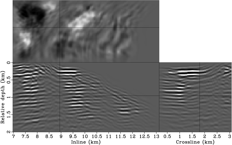
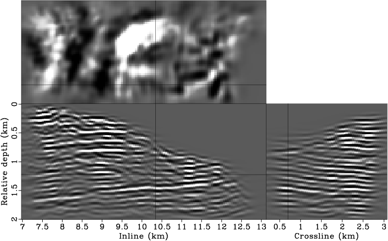
Figure 8. The migrated image of the 3-D GOM data set. Panels (a) and (b) show different slices of the same 3-D cube. The image has been masked using the mask operator shown in Figure 7 to focus on comparing sediment reflectivities. [CR]

lsm3d-noreg-invt1,lsm3d-noreg-invt2
Figure 9. The inverted image without applying any regularization. Panels (a) and (b) show different slices of the same 3-D cube. [CR]

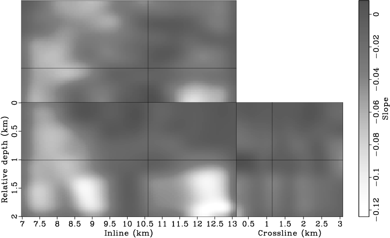
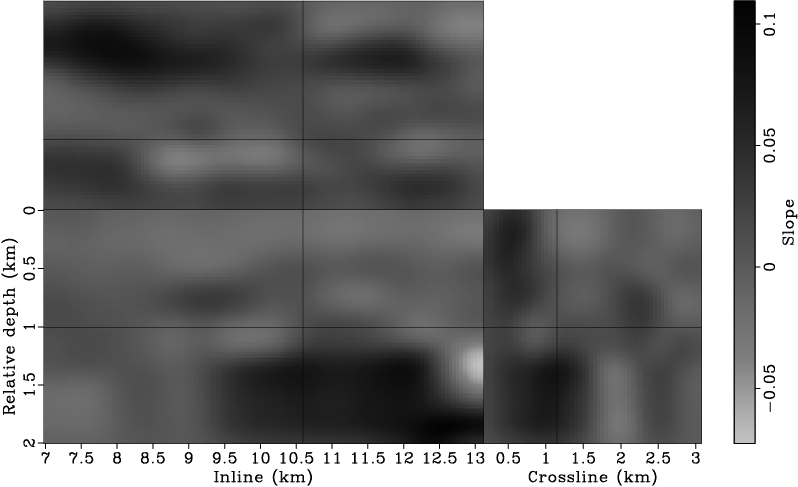
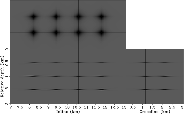
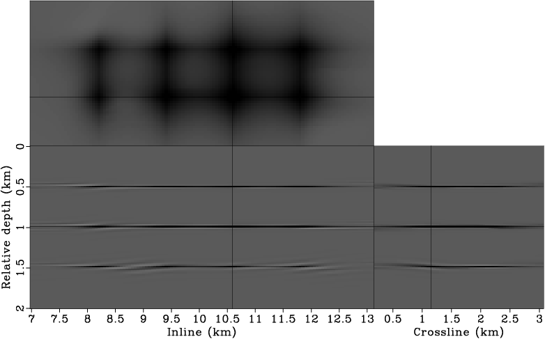
In order to regularize the inversion with a reasonably accurate model covariance, we interpret the migrated image and manually pick several key reflectors (Figure 10). We estimate dip fields based on the interpreted reflectors using the structure tensor method (Hale, 2007; van Vliet and Verbeek, 1995). The estimated dips have been smoothed with a triangle filter and are shown in Figure 11. The dip field is then used to build a bank of dip filters for preconditioning. Figures 12, 13 and 14 show impulse responses of the dip filters as smoothing strength increases. Note that the stronger the smoothing effect, the longer the filter response. These dip filters also vary spatially, and each dip filter smooths along a direction conformal to the corresponding dip values.

lsm3d-refl-pick
Figure 10. Interpreted horizons from the migrated image. The horizons are then used to build the dip field for dip filtering. [CR]

lsm3d-dipx-pick,lsm3d-dipy-pick
Figure 11. The estimated dip field from the interpreted reflectors. Panels (a) and (b) are the slopes in the inline and crossline directions, respectively. [CR]

lsm3d-dipflt3
Figure 12. Impulse responses of the dip filters with weak smoothing. [CR]

lsm3d-dipflt1
Figure 13. Impulse responses of the dip filters with moderate smoothing. [CR]

lsm3d-dipflt6
Figure 14. Impulse responses of the dip filters with strong smoothing. [CR]

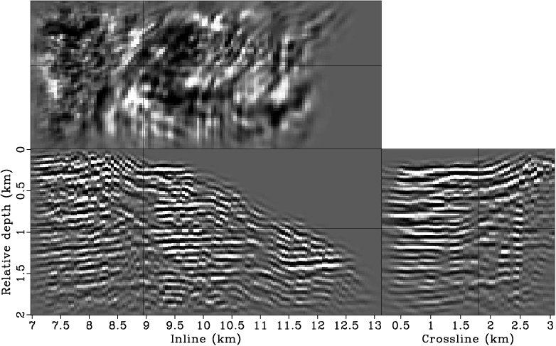
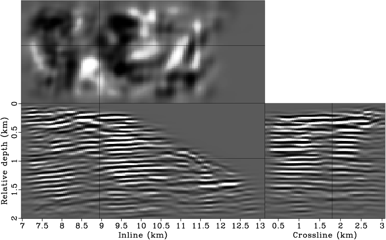
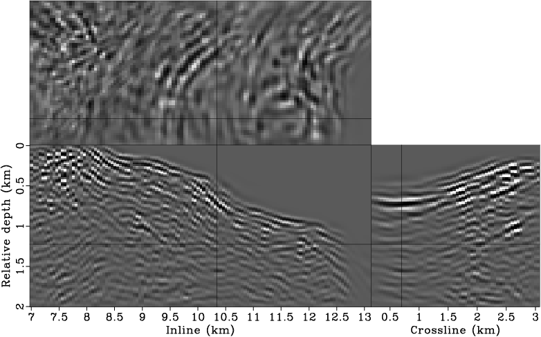
Figure 15 presents the inverted image after $100$ iterations when preconditioned by the dip filter with weak smoothing (Figure 12). The result is significantly improved over the one obtained without any regularizations (Figure 9). The reflectors are much more coherent and they extend further into the shadow zone, filling in the illumination gap almost completely. The regularized image is much easier to interpret geologically.

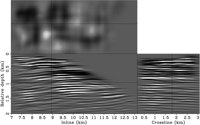
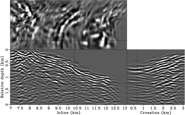
To see the effects of regularization (or preconditioning), we increase the smoothing strength of the dip filters. Figure 16 shows the inversion result after $100$ iterations when we use dip filters with moderate smoothing (Figure 12) for preconditioning. The result further enhances the coherence and continuity of the reflectors and the inverted image looks even cleaner. However, the spatial resolution of the image seems somewhat degraded by the smoothing effect of the preconditioner (This becomes clear by comparing the depth slices of Figures 9, 15 and 16).

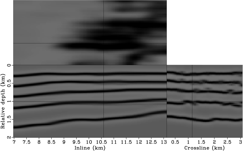
Figure 17 shows the inversion result when we further increase the smoothing strength of the dip filters (Figure 14). In this extreme case, inversion is dominated by preconditioning. The inverted image honors the user-supplied model-covariance, but not necessarily the data. (The data fitting plays little role in this case.)

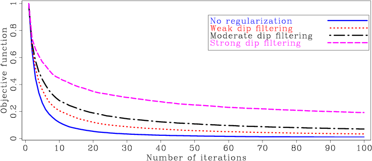
Figures 18 and 19 compare the residuals at the last iteration and the convergence of objective functions for different methods. As expected, inversion without any regularization, which fits the data most closely, has the smallest residual, whereas inversion preconditioned with strong dip filters, which fits the data least closely, has the biggest residual.

lsm3d-a-invt1,lsm3d-a-invt2
Figure 15. The inverted image when preconditioned using dip filters with weak smoothing (Figure 12). [CR]

lsm3d-b-invt1,lsm3d-b-invt2
Figure 16. The inverted image when preconditioned using dip filters with moderate smoothing (Figure 13). [CR]

lsm3d-c-invt1,lsm3d-c-invt2
Figure 17. The inverted image when preconditioned using dip filters with strong smoothing (Figure 14). [CR]

lsm3d-noreg-resd,lsm3d-a-resd,lsm3d-b-resd,lsm3d-c-resd
Figure 18. Residuals at the last iteration for different methods. Panel (a) is obtained using inversion without regularization. Panels (b), (c) and (d) are obtained using inversion preconditioned with weak, moderate and strong dip filtering, respectively. All panels are clipped to the same value. [CR]

lsm3d-fobj
Figure 19. Evolution of objective functions for different inversion methods. [CR]

Subsalt imaging by target-oriented wavefield least-squares migration: A 3-D field-data example