|
 |
 |
 | Subsalt imaging by target-oriented wavefield least-squares migration: A 3-D field-data example |  |
![[pdf]](icons/pdf.png) |
Next: About this document ...
Up: Tang and Biondi: 3-D
Previous: Acknowledgements
-
Ayeni, G., Y. Tang, and B. Biondi, 2009, Joint preconditioned least-squares
inversion of simultaneous source time-lapse seismic data sets: SEG Technical
Program Expanded Abstracts, 28, 3914-3918.
-
-
Biondi, B., S. Fomel, and N. Chemingui, 1998, Azimuth moveout for 3-d prestack
imaging: Geophysics, 63, 574-588.
-
-
Claerbout, J., 1998, Multidimensional recursive filters via a helix:
Geophysics, 63, 1532-1541.
-
-
Claerbout, J. F., 1985, Imaging the earth's interior: Blackwell Scientific
Publication.
-
-
----, 1992, Earth soundings analysis: Processing versus inversion:
Blackwell Scientific Publication.
-
-
----, 2008, Image Estimation By Example: Geophysical Sounding
Image Construction: Multidimensional Autoregression: Stanford
University.
-
-
Clapp, M. L., 2005, Imaging Under Salt: Illumination Compensation by
Regularized Inversion: PhD thesis, Stanford University.
-
-
Clapp, R., 2003, Geologically Constrained Migration Velocity Analysis:
PhD thesis, Stanford University.
-
-
Duquet, B., P. Lailly, and A. Ehinger, 2001, 3d plane wave migration of
streamer data: SEG Technical Program Expanded Abstracts, 20,
1033-1036.
-
-
Fomel, S., P. Sava, J. Rickett, and J. F. Claerbout, 2003, The wilson–burg
method of spectral factorization with application to helical filtering:
Geophysical Prospecting, 51, 409-420.
-
-
Gray, R. and L. D. Davisson, 2003, Introduction to Statistical Signal
Processing: Cambridge University Press.
-
-
Hale, D., 2007, Local dip filtering with directional laplacians: CWP Project
Review, 567, 91-102.
-
-
Kühl, H. and M. D. Sacchi, 2003, Least-squares wave-equation migration for
avp/ava inversion: Geophysics, 68, 262-273.
-
-
Lailly, P., 1983, The seismic inverse problem as a sequence of before stack
migration: Proc. Conf. on Inverse Scattering, Theory and Applications,
Expanded Abstracts, Philadelphia, SIAM.
-
-
Lecomte, I., 2008, Resolution and illumination analyses in PSDM: A ray-based
approach: The Leading Edge, 27, no. 5, 650-663.
-
-
Liu, F., D. W. Hanson, N. D. Whitmore, R. S. Day, and R. H. Stolt, 2006,
Toward a unified analysis for source plane-wave migration: Geophysics, 71, no. 4, S129-S139.
-
-
Nemeth, T., C. Wu, and G. T. Schuster, 1999, Least-squares migration of
incomplete reflection data: Geophysics, 64, 208-221.
-
-
Stolt, R. H. and A. Benson, 1986, Seismic Migration: Theory and
Practice: Geophysical Press.
-
-
Tang, Y., 2009, Target-oriented wave-equation least-squares
migration/inversion with phase-encoded Hessian: Geophysics, 74,
WCA95-WCA107.
-
-
Tang, Y. and B. Biondi, 2011, Subsalt velocity analysis by target-oriented
wavefield tomography: A 3-D field-data example: SEP-143, xxx-xxx.
-
-
Tang, Y. and S. Lee, 2010, Preconditioning full waveform inversion with
phase-encoded hessian: SEG Technical Program Expanded Abstracts, 29,
1034-1038.
-
-
Valenciano, A., 2008, Imaging by Wave-equation Inversion: PhD thesis,
Stanford University.
-
-
van Vliet, L. J. and P. W. Verbeek, 1995, Estimators for orientation and
anisotropy in digitized images: ASCI’95, Proc. First Annual Conference of
the Advanced School for Computing and Imaging (Heijen, NL, May 16-18), ASCI,
442-450.
-
-
Whitmore, N. D., 1995, An Imaging Hierarchy for Common Angle Plane
Wave Seismogram: PhD thesis, University of Tulsa.
-
-
Zhang, Y., J. Sun, C. Notfors, S. H. Gray, L. Chernis, and J. Young, 2005,
Delayed-shot 3d depth migration: Geophysics, 70, E21-E28.
-
Appendix
A
3-D conical-wave domain Hessian
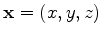
In general, a 3-D surface seismic data set can be represented by a 5-D object
 , with
 and
and
 being the receiver and source position, respectively,
and
being the receiver and source position, respectively,
and  being the angular frequency. Under the Born approximation (Stolt and Benson, 1986),
the data can be modeled by a linear
operator as follows:
being the angular frequency. Under the Born approximation (Stolt and Benson, 1986),
the data can be modeled by a linear
operator as follows:
 |
|
|
(17) |
where 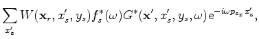 is the source function;
 and
and
 are the Green's functions
connecting the source and receiver position to the image point
are the Green's functions
connecting the source and receiver position to the image point
 , respectively.
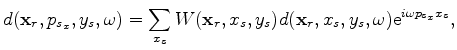
We can transform data into the conical-wave domain by
slant-stacking along the inline source axis
, respectively.
We can transform data into the conical-wave domain by
slant-stacking along the inline source axis  as follows:
 |
|
|
(18) |
where
 is the acquisition mask operator, which contains ones where we record data, and zeros where we do not;
 is the surface ray parameter in the inline direction.
The inverse transform is
is the surface ray parameter in the inline direction.
The inverse transform is
 |
|
|
(19) |
where 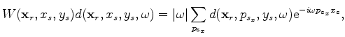 on the right hand side of the equation is also known as the ``rho'' filter (Claerbout, 1985).
To find a reflectivity model  that best fits the observed data for a given background velocity,
we can minimize a data-misfit function that measures the differences between the observed data
and the synthesized data in a least-squares sense.
In the point-source case, the data-misfit function is
that best fits the observed data for a given background velocity,
we can minimize a data-misfit function that measures the differences between the observed data
and the synthesized data in a least-squares sense.
In the point-source case, the data-misfit function is
![$\displaystyle F({\bf m}) = \frac{1}{2}\sum_{\omega}\sum_{{\bf x}_s}\sum_{{\bf x...
...[d({\bf x}_r,{\bf x}_s,\omega)-d_{\rm obs}({\bf x}_r,{\bf x}_s,\omega)]\vert^2,$](img122.png) |
|
|
(20) |
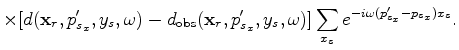
where 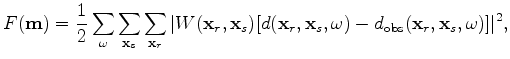 is the observed data. Substituting equation A-3 into A-4 yields
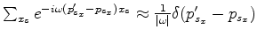
If the inline source axis  is reasonably well sampled, we have
 ,
where
,
where  is the Dirac delta function.
Therefore,
an objective function equivalent to equation A-4 in the 3-D conical-wave domain takes the following form:
is the Dirac delta function.
Therefore,
an objective function equivalent to equation A-4 in the 3-D conical-wave domain takes the following form:
 |
|
|
(22) |
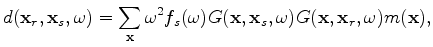
The Hessian operator in the 3-D conical-wave domain can be obtained by taking the second-order derivatives
of 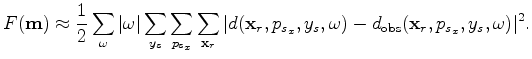 (equation A-6) with respect to the model parameters:
 |
|
|
(23) |
When
 , we obtain the diagonal components of the Hessian,
which are also known as the subsurface illumination;
otherwise, we obtain the off-diagonal components of the Hessian, which
are also known as the resolution function for a given acquisition setup.
, we obtain the diagonal components of the Hessian,
which are also known as the subsurface illumination;
otherwise, we obtain the off-diagonal components of the Hessian, which
are also known as the resolution function for a given acquisition setup.
With equations A-1 and A-2,
we obtain the expression of the derivative of 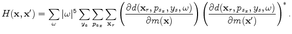 with respect to
  as follows:
Substituting equation A-8 into equation A-7 yields the expression
for each component of the Hessian matrix in the 3-D conical-wave domain:
|
|
|
|
| Subsalt imaging by target-oriented wavefield least-squares migration: A 3-D field-data example | |
|
Next: About this document ...
Up: Tang and Biondi: 3-D
Previous: Acknowledgements
2011-05-24
![$\displaystyle \times [d({\bf x}_r,p_{s_x} ,y_s,\omega)-d_{\rm obs}({\bf x}_r,p_{s_x} ,y_s,\omega)]^{*}$](img126.png)